Linear–Quadratic Optimal Control and the Riccati Differential Equation
The preceding sections derived the state equation, costate equation, stationarity condition, endpoint constraints, and transversality conditions for a general optimal-control problem. This section applies those necessary conditions to one of the most important analytically tractable problems in control theory: the finite-horizon linear–quadratic regulator (LQR).
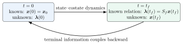
The LQR problem is important for two reasons. First, it provides a complete example in which the optimality conditions can be reduced to a computable feedback law. Second, it exposes a central difficulty of indirect optimal control: the state and costate equations form a two-point boundary-value problem, with state information specified at the initial time and costate information specified at the final time.
The finite-horizon LQR problem ¶ Consider the linear time-invariant system
x ˙ ( t ) = A x ( t ) + B u ( t ) , x ( 0 ) = x 0 , \dot{\boldsymbol{x}}(t)=A\boldsymbol{x}(t)+B\boldsymbol{u}(t),
\qquad
\boldsymbol{x}(0)=\boldsymbol{x}_0, x ˙ ( t ) = A x ( t ) + B u ( t ) , x ( 0 ) = x 0 , where x ( t ) ∈ R n \boldsymbol{x}(t)\in\mathbb{R}^n x ( t ) ∈ R n u ( t ) ∈ R m \boldsymbol{u}(t)\in\mathbb{R}^m u ( t ) ∈ R m A ∈ R n × n A\in\mathbb{R}^{n\times n} A ∈ R n × n B ∈ R n × m B\in\mathbb{R}^{n\times m} B ∈ R n × m
The finite-horizon LQR problem is
min u ( ⋅ ) J = 1 2 x T ( t f ) S f x ( t f ) + 1 2 ∫ 0 t f [ x T ( t ) Q x ( t ) + u T ( t ) R u ( t ) ] d t , \begin{aligned}
\min_{\boldsymbol{u}(\cdot)}\quad
J
&=
\frac{1}{2}\boldsymbol{x}^{\mathsf{T}}(t_f)S_f\boldsymbol{x}(t_f)
+
\frac{1}{2}\int_{0}^{t_f}
\left[
\boldsymbol{x}^{\mathsf{T}}(t)Q\boldsymbol{x}(t)
+
\boldsymbol{u}^{\mathsf{T}}(t)R\boldsymbol{u}(t)
\right]\,\mathrm{d} t,
\end{aligned} u ( ⋅ ) min J = 2 1 x T ( t f ) S f x ( t f ) + 2 1 ∫ 0 t f [ x T ( t ) Q x ( t ) + u T ( t ) R u ( t ) ] d t , subject to x ˙ ( t ) = A x ( t ) + B u ( t ) , x ( 0 ) = x 0 . \begin{aligned}
\text{subject to}\quad
\dot{\boldsymbol{x}}(t)&=A\boldsymbol{x}(t)+B\boldsymbol{u}(t),
\qquad
\boldsymbol{x}(0)=\boldsymbol{x}_0.
\end{aligned} subject to x ˙ ( t ) = A x ( t ) + B u ( t ) , x ( 0 ) = x 0 . The final state is free; it is penalized rather than prescribed.
The standard weighting assumptions are
Q = Q T ⪰ 0 , R = R T ≻ 0 , S f = S f T ⪰ 0. Q=Q^{\mathsf{T}}\succeq 0,
\qquad
R=R^{\mathsf{T}}\succ 0,
\qquad
S_f=S_f^{\mathsf{T}}\succeq 0. Q = Q T ⪰ 0 , R = R T ≻ 0 , S f = S f T ⪰ 0. The matrices may be time varying in the general finite-horizon problem. This section assumes constant A A A B B B Q Q Q R R R
Interpretation of the quadratic cost ¶ The running cost contains two competing penalties:
1 2 x T Q x and 1 2 u T R u . \frac{1}{2}\boldsymbol{x}^{\mathsf{T}} Q\boldsymbol{x}
\qquad\text{and}\qquad
\frac{1}{2}\boldsymbol{u}^{\mathsf{T}} R\boldsymbol{u}. 2 1 x T Q x and 2 1 u T R u . The first penalizes undesirable state deviations, while the second penalizes control effort. The terminal term 1 2 x T ( t f ) S f x ( t f ) \tfrac12\boldsymbol{x}^{\mathsf{T}}(t_f)S_f\boldsymbol{x}(t_f) 2 1 x T ( t f ) S f x ( t f )
Controllability and observability assumptions ¶ A common strong set of assumptions is that ( A , B ) (A,B) ( A , B ) ( A , Q 1 / 2 ) (A,Q^{1/2}) ( A , Q 1/2 )
Because Q ⪰ 0 Q\succeq0 Q ⪰ 0
Q = C T C , Q=C^{\mathsf{T}} C, Q = C T C , For example, with C = Q 1 / 2 C=Q^{1/2} C = Q 1/2
x T Q x = ∥ C x ∥ 2 2 . \boldsymbol{x}^{\mathsf{T}} Q\boldsymbol{x}=\|C\boldsymbol{x}\|_2^2. x T Q x = ∥ C x ∥ 2 2 . Observability or detectability of ( A , C ) (A,C) ( A , C ) ( A , Q ) (A,Q) ( A , Q ) ( A , Q 1 / 2 ) (A,Q^{1/2}) ( A , Q 1/2 )
The Mayer term and running cost are
Φ = 1 2 x T ( t f ) S f x ( t f ) , L = 1 2 x T Q x + 1 2 u T R u . \Phi=\frac12\boldsymbol{x}^{\mathsf{T}}(t_f)S_f\boldsymbol{x}(t_f),
\qquad
L=\frac12\boldsymbol{x}^{\mathsf{T}} Q\boldsymbol{x}+\frac12\boldsymbol{u}^{\mathsf{T}} R\boldsymbol{u}. Φ = 2 1 x T ( t f ) S f x ( t f ) , L = 2 1 x T Q x + 2 1 u T R u . The dynamics are
f ( x , u ) = A x + B u . \boldsymbol{f}(\boldsymbol{x},\boldsymbol{u})=A\boldsymbol{x}+B\boldsymbol{u}. f ( x , u ) = A x + B u . Therefore, the Hamiltonian is
H ( x , u , λ ) = 1 2 x T Q x + 1 2 u T R u + λ T ( A x + B u ) . H(\boldsymbol{x},\boldsymbol{u},\boldsymbol{\lambda})
=
\frac12\boldsymbol{x}^{\mathsf{T}} Q\boldsymbol{x}
+
\frac12\boldsymbol{u}^{\mathsf{T}} R\boldsymbol{u}
+
\boldsymbol{\lambda}^{\mathsf{T}}(A\boldsymbol{x}+B\boldsymbol{u}). H ( x , u , λ ) = 2 1 x T Q x + 2 1 u T R u + λ T ( A x + B u ) . Step 2: Derive the costate equation ¶ The costate equation is
λ ˙ = − H x T . \dot{\boldsymbol{\lambda}}=-H_{\boldsymbol{x}}^{\mathsf{T}}. λ ˙ = − H x T . Because Q = Q T Q=Q^{\mathsf{T}} Q = Q T
∂ ∂ x ( 1 2 x T Q x ) = x T Q . \frac{\partial}{\partial\boldsymbol{x}}
\left(\frac12\boldsymbol{x}^{\mathsf{T}} Q\boldsymbol{x}\right)
=
\boldsymbol{x}^{\mathsf{T}} Q. ∂ x ∂ ( 2 1 x T Q x ) = x T Q . Also,
∂ ∂ x ( λ T A x ) = λ T A . \frac{\partial}{\partial\boldsymbol{x}}
\left(\boldsymbol{\lambda}^{\mathsf{T}} A\boldsymbol{x}\right)
=
\boldsymbol{\lambda}^{\mathsf{T}} A. ∂ x ∂ ( λ T A x ) = λ T A . Thus,
H x = x T Q + λ T A , H_{\boldsymbol{x}}=\boldsymbol{x}^{\mathsf{T}} Q+\boldsymbol{\lambda}^{\mathsf{T}} A, H x = x T Q + λ T A , and therefore
λ ˙ = − Q x − A T λ . \boxed{
\dot{\boldsymbol{\lambda}}=-Q\boldsymbol{x}-A^{\mathsf{T}}\boldsymbol{\lambda}.
} λ ˙ = − Q x − A T λ . Step 3: Determine the stationary control ¶ The control is unconstrained, so the minimizing control lies in the interior of the admissible control set. The stationarity condition is therefore
H u = 0 T . H_{\boldsymbol{u}}=\boldsymbol{0}^{\mathsf{T}}. H u = 0 T . Differentiating (12) u \boldsymbol{u} u
H u = u T R + λ T B . H_{\boldsymbol{u}}=\boldsymbol{u}^{\mathsf{T}} R+\boldsymbol{\lambda}^{\mathsf{T}} B. H u = u T R + λ T B . Taking the transpose and setting the result equal to zero yields
R u + B T λ = 0 . R\boldsymbol{u}+B^{\mathsf{T}}\boldsymbol{\lambda}=\boldsymbol{0}. R u + B T λ = 0 . Since R ≻ 0 R\succ0 R ≻ 0
u ∗ = − R − 1 B T λ . \boxed{
\boldsymbol{u}^*=-R^{-1}B^{\mathsf{T}}\boldsymbol{\lambda}.
} u ∗ = − R − 1 B T λ . The equation H u = 0 H_{\boldsymbol{u}}=0 H u = 0 u \boldsymbol{u} u H u = 0 H_{\boldsymbol{u}}=0 H u = 0
The coupled state–costate system ¶ Substituting (21)
x ˙ = A x − B R − 1 B T λ . \dot{\boldsymbol{x}}
=A\boldsymbol{x}-BR^{-1}B^{\mathsf{T}}\boldsymbol{\lambda}. x ˙ = A x − B R − 1 B T λ . Together with (17)
λ ˙ = − Q x − A T λ . \dot{\boldsymbol{\lambda}}=-Q\boldsymbol{x}-A^{\mathsf{T}}\boldsymbol{\lambda}. λ ˙ = − Q x − A T λ . These equations may be assembled as
[ x ˙ λ ˙ ] = [ A − B R − 1 B T − Q − A T ] ⏟ H [ x λ ] . \boxed{
\begin{bmatrix}
\dot{\boldsymbol{x}}\\[1mm]
\dot{\boldsymbol{\lambda}}
\end{bmatrix}
=
\underbrace{
\begin{bmatrix}
A & -BR^{-1}B^{\mathsf{T}}\\
-Q & -A^{\mathsf{T}}
\end{bmatrix}}_{\displaystyle \mathcal{H}}
\begin{bmatrix}
\boldsymbol{x}\\[1mm]
\boldsymbol{\lambda}
\end{bmatrix}.
} [ x ˙ λ ˙ ] = H [ A − Q − B R − 1 B T − A T ] [ x λ ] . The matrix H ∈ R 2 n × 2 n \mathcal{H}\in\mathbb{R}^{2n\times2n} H ∈ R 2 n × 2 n
Although this expression is formally complete, it does not yet solve the optimal-control problem because λ ( 0 ) \boldsymbol{\lambda}(0) λ ( 0 )
Endpoint conditions ¶ Initial endpoint ¶ The initial condition may be represented as the endpoint constraint
ϕ = x ( 0 ) − x 0 = 0 . \boldsymbol{\phi}=\boldsymbol{x}(0)-\boldsymbol{x}_0=\boldsymbol{0}. ϕ = x ( 0 ) − x 0 = 0 . Because the initial state is fixed,
δ x ( 0 ) = 0 . \delta\boldsymbol{x}(0)=\boldsymbol{0}. δ x ( 0 ) = 0 . Consequently, the initial transversality condition does not provide a useful numerical condition on λ ( 0 ) \boldsymbol{\lambda}(0) λ ( 0 ) (28)
Final endpoint ¶ The final state is free, so the terminal transversality condition applies:
λ ( t f ) = Φ x ( t f ) T . \boldsymbol{\lambda}(t_f)=\Phi_{\boldsymbol{x}(t_f)}^{\mathsf{T}}. λ ( t f ) = Φ x ( t f ) T . Since
Φ = 1 2 x T ( t f ) S f x ( t f ) \Phi=\frac12\boldsymbol{x}^{\mathsf{T}}(t_f)S_f\boldsymbol{x}(t_f) Φ = 2 1 x T ( t f ) S f x ( t f ) and S f = S f T S_f=S_f^{\mathsf{T}} S f = S f T
λ ( t f ) = S f x ( t f ) . \boxed{
\boldsymbol{\lambda}(t_f)=S_f\boldsymbol{x}(t_f).
} λ ( t f ) = S f x ( t f ) . The complete boundary data are therefore
x ( 0 ) = x 0 , λ ( t f ) = S f x ( t f ) . \boxed{
\boldsymbol{x}(0)=\boldsymbol{x}_0,
\qquad
\boldsymbol{\lambda}(t_f)=S_f\boldsymbol{x}(t_f).
} x ( 0 ) = x 0 , λ ( t f ) = S f x ( t f ) . There are n n n n n n 2 n 2n 2 n (24)
The two-point boundary-value problem ¶ Equations (24) (33)
x ˙ = A x − B R − 1 B T λ , x ( 0 ) = x 0 , \begin{aligned}
\dot{\boldsymbol{x}}&=A\boldsymbol{x}-BR^{-1}B^{\mathsf{T}}\boldsymbol{\lambda},
&\boldsymbol{x}(0)&=\boldsymbol{x}_0,
\end{aligned} x ˙ = A x − B R − 1 B T λ , x ( 0 ) = x 0 , λ ˙ = − Q x − A T λ , λ ( t f ) = S f x ( t f ) . \begin{aligned}
\dot{\boldsymbol{\lambda}}&=-Q\boldsymbol{x}-A^{\mathsf{T}}\boldsymbol{\lambda},
&\boldsymbol{\lambda}(t_f)&=S_f\boldsymbol{x}(t_f).
\end{aligned} λ ˙ = − Q x − A T λ , λ ( t f ) = S f x ( t f ) . The difficulty is structural: the full vector [ x T , λ T ] T [\boldsymbol{x}^{\mathsf{T}},\boldsymbol{\lambda}^{\mathsf{T}}]^{\mathsf{T}} [ x T , λ T ] T
Figure 1: Boundary information for finite-horizon LQR is split between the initial state and terminal costate relation.
A direct matrix-exponential representation is possible. Partition the state-transition matrix as
e H t f = [ Ψ 11 Ψ 12 Ψ 21 Ψ 22 ] . e^{\mathcal{H}t_f}
=
\begin{bmatrix}
\Psi_{11} & \Psi_{12}\\
\Psi_{21} & \Psi_{22}
\end{bmatrix}. e H t f = [ Ψ 11 Ψ 21 Ψ 12 Ψ 22 ] . Then
[ x ( t f ) λ ( t f ) ] = [ Ψ 11 Ψ 12 Ψ 21 Ψ 22 ] [ x 0 λ ( 0 ) ] . \begin{bmatrix}
\boldsymbol{x}(t_f)\\
\boldsymbol{\lambda}(t_f)
\end{bmatrix}
=
\begin{bmatrix}
\Psi_{11} & \Psi_{12}\\
\Psi_{21} & \Psi_{22}
\end{bmatrix}
\begin{bmatrix}
\boldsymbol{x}_0\\
\boldsymbol{\lambda}(0)
\end{bmatrix}. [ x ( t f ) λ ( t f ) ] = [ Ψ 11 Ψ 21 Ψ 12 Ψ 22 ] [ x 0 λ ( 0 ) ] . Using λ ( t f ) = S f x ( t f ) \boldsymbol{\lambda}(t_f)=S_f\boldsymbol{x}(t_f) λ ( t f ) = S f x ( t f )
( Ψ 22 − S f Ψ 12 ) λ ( 0 ) = ( S f Ψ 11 − Ψ 21 ) x 0 . \left(\Psi_{22}-S_f\Psi_{12}\right)\boldsymbol{\lambda}(0)
=
\left(S_f\Psi_{11}-\Psi_{21}\right)\boldsymbol{x}_0. ( Ψ 22 − S f Ψ 12 ) λ ( 0 ) = ( S f Ψ 11 − Ψ 21 ) x 0 . If the matrix on the left is nonsingular, (38) λ ( 0 ) \boldsymbol{\lambda}(0) λ ( 0 )
Motivated by the linear structure of the problem, introduce
λ ( t ) = S ( t ) x ( t ) + β ( t ) , \boxed{
\boldsymbol{\lambda}(t)=S(t)\boldsymbol{x}(t)+\boldsymbol{\beta}(t),
} λ ( t ) = S ( t ) x ( t ) + β ( t ) , where S ( t ) ∈ R n × n S(t)\in\mathbb{R}^{n\times n} S ( t ) ∈ R n × n β ( t ) ∈ R n \boldsymbol{\beta}(t)\in\mathbb{R}^n β ( t ) ∈ R n
This transformation initially loses no generality because β ( t ) \boldsymbol{\beta}(t) β ( t ) S ( t ) S(t) S ( t ) β \boldsymbol{\beta} β
Differentiating (39)
λ ˙ = S ˙ x + S x ˙ + β ˙ . \dot{\boldsymbol{\lambda}}=\dot{S}\boldsymbol{x}+S\dot{\boldsymbol{x}}+\dot{\boldsymbol{\beta}}. λ ˙ = S ˙ x + S x ˙ + β ˙ . Using
x ˙ = A x − B R − 1 B T ( S x + β ) , \dot{\boldsymbol{x}}=A\boldsymbol{x}-BR^{-1}B^{\mathsf{T}}(S\boldsymbol{x}+\boldsymbol{\beta}), x ˙ = A x − B R − 1 B T ( S x + β ) , we obtain
λ ˙ = ( S ˙ + S A − S B R − 1 B T S ) x + β ˙ − S B R − 1 B T β . \begin{aligned}
\dot{\boldsymbol{\lambda}}
={}&
\left(
\dot{S}+SA-SBR^{-1}B^{\mathsf{T}} S
\right)\boldsymbol{x}
\nonumber\\
&+
\dot{\boldsymbol{\beta}}-SBR^{-1}B^{\mathsf{T}}\boldsymbol{\beta}.
\end{aligned} λ ˙ = ( S ˙ + S A − SB R − 1 B T S ) x + β ˙ − SB R − 1 B T β . On the other hand, the costate equation gives
λ ˙ = − Q x − A T ( S x + β ) = ( − Q − A T S ) x − A T β . \begin{aligned}
\dot{\boldsymbol{\lambda}}
&=-Q\boldsymbol{x}-A^{\mathsf{T}}(S\boldsymbol{x}+\boldsymbol{\beta})
\nonumber\\
&=
\left(-Q-A^{\mathsf{T}} S\right)\boldsymbol{x}-A^{\mathsf{T}}\boldsymbol{\beta}.
\end{aligned} λ ˙ = − Q x − A T ( S x + β ) = ( − Q − A T S ) x − A T β . Equating (42) (43)
β ˙ = [ − S ˙ − S A − A T S + S B R − 1 B T S − Q ] x + ( S B R − 1 B T − A T ) β . \begin{aligned}
\dot{\boldsymbol{\beta}}
={}&
\Bigl[
-\dot{S}-SA-A^{\mathsf{T}} S
+SBR^{-1}B^{\mathsf{T}} S-Q
\Bigr]\boldsymbol{x}
\nonumber\\
&+
\left(SBR^{-1}B^{\mathsf{T}}-A^{\mathsf{T}}\right)\boldsymbol{\beta}.
\end{aligned} β ˙ = [ − S ˙ − S A − A T S + SB R − 1 B T S − Q ] x + ( SB R − 1 B T − A T ) β . Define the matrix residual
Γ ( S ) = − S ˙ − S A − A T S + S B R − 1 B T S − Q . \Gamma(S)
=
-\dot{S}-SA-A^{\mathsf{T}} S+SBR^{-1}B^{\mathsf{T}} S-Q. Γ ( S ) = − S ˙ − S A − A T S + SB R − 1 B T S − Q . Then
β ˙ = Γ ( S ) x + ( S B R − 1 B T − A T ) β . \dot{\boldsymbol{\beta}}
=
\Gamma(S)\boldsymbol{x}+
\left(SBR^{-1}B^{\mathsf{T}}-A^{\mathsf{T}}\right)\boldsymbol{\beta}. β ˙ = Γ ( S ) x + ( SB R − 1 B T − A T ) β . The Riccati differential equation ¶ Choose S ( t ) S(t) S ( t )
Γ ( S ) = 0. \Gamma(S)=0. Γ ( S ) = 0. This eliminates the state forcing from the β \boldsymbol{\beta} β
− S ˙ = A T S + S A − S B R − 1 B T S + Q . \boxed{
-\dot{S}
=A^{\mathsf{T}} S+SA-SBR^{-1}B^{\mathsf{T}} S+Q.
} − S ˙ = A T S + S A − SB R − 1 B T S + Q . Equivalently,
Equation (48)
Terminal conditions for the Riccati matrix and auxiliary vector ¶ At t = t f t=t_f t = t f (39)
λ ( t f ) = S ( t f ) x ( t f ) + β ( t f ) . \boldsymbol{\lambda}(t_f)=S(t_f)\boldsymbol{x}(t_f)+\boldsymbol{\beta}(t_f). λ ( t f ) = S ( t f ) x ( t f ) + β ( t f ) . The transversality condition requires
λ ( t f ) = S f x ( t f ) . \boldsymbol{\lambda}(t_f)=S_f\boldsymbol{x}(t_f). λ ( t f ) = S f x ( t f ) . A natural choice consistent for every terminal state is therefore
S ( t f ) = S f , β ( t f ) = 0 . \boxed{
S(t_f)=S_f,
\qquad
\boldsymbol{\beta}(t_f)=\boldsymbol{0}.
} S ( t f ) = S f , β ( t f ) = 0 . Once S S S (46)
β ˙ = ( S B R − 1 B T − A T ) β . \dot{\boldsymbol{\beta}}
=
\left(SBR^{-1}B^{\mathsf{T}}-A^{\mathsf{T}}\right)\boldsymbol{\beta}. β ˙ = ( SB R − 1 B T − A T ) β . This is a homogeneous linear differential equation. Because β ( t f ) = 0 \boldsymbol{\beta}(t_f)=0 β ( t f ) = 0
β ( t ) ≡ 0 for all t ∈ [ 0 , t f ] . \boxed{
\boldsymbol{\beta}(t)\equiv\boldsymbol{0}
\qquad\text{for all }t\in[0,t_f].
} β ( t ) ≡ 0 for all t ∈ [ 0 , t f ] . Hence,
λ ( t ) = S ( t ) x ( t ) . \boxed{
\boldsymbol{\lambda}(t)=S(t)\boldsymbol{x}(t).
} λ ( t ) = S ( t ) x ( t ) . The zero result is specific to the regulator problem with no affine dynamics, no reference-tracking terms, and no linear terms in the cost. In tracking and affine optimal-control problems, β ( t ) \boldsymbol{\beta}(t) β ( t )
Optimal feedback law ¶ Substituting (57) (21)
u ∗ ( t ) = − R − 1 B T S ( t ) x ∗ ( t ) . \boldsymbol{u}^*(t)
=-R^{-1}B^{\mathsf{T}} S(t)\boldsymbol{x}^*(t). u ∗ ( t ) = − R − 1 B T S ( t ) x ∗ ( t ) . Define the time-varying gain
K ( t ) = R − 1 B T S ( t ) . \boxed{
K(t)=R^{-1}B^{\mathsf{T}} S(t).
} K ( t ) = R − 1 B T S ( t ) . Then
u ∗ ( t ) = − K ( t ) x ∗ ( t ) . \boxed{
\boldsymbol{u}^*(t)=-K(t)\boldsymbol{x}^*(t).
} u ∗ ( t ) = − K ( t ) x ∗ ( t ) . The optimal state satisfies the closed-loop equation
x ˙ ∗ ( t ) = [ A − B K ( t ) ] x ∗ ( t ) , x ∗ ( 0 ) = x 0 . \boxed{
\dot{\boldsymbol{x}}^*(t)
=
\left[A-BK(t)\right]\boldsymbol{x}^*(t),
\qquad
\boldsymbol{x}^*(0)=\boldsymbol{x}_0.
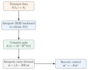
} x ˙ ∗ ( t ) = [ A − B K ( t ) ] x ∗ ( t ) , x ∗ ( 0 ) = x 0 . Figure 2: Backward–forward computational workflow for finite-horizon linear–quadratic optimal control.
Backward–forward computational procedure ¶ The Riccati formulation converts the original TPBVP into two sequential initial/terminal-value integrations:
Specify A A A B B B Q Q Q R R R S f S_f S f t f t_f t f x 0 \boldsymbol{x}_0 x 0
Integrate the RDE
− S ˙ = A T S + S A − S B R − 1 B T S + Q -\dot{S}=A^{\mathsf{T}} S+SA-SBR^{-1}B^{\mathsf{T}} S+Q − S ˙ = A T S + S A − SB R − 1 B T S + Q backward from S ( t f ) = S f S(t_f)=S_f S ( t f ) = S f t = 0 t=0 t = 0
Compute K ( t ) = R − 1 B T S ( t ) K(t)=R^{-1}B^{\mathsf{T}} S(t) K ( t ) = R − 1 B T S ( t )
Integrate
x ˙ ∗ = [ A − B K ( t ) ] x ∗ , x ∗ ( 0 ) = x 0 , \dot{\boldsymbol{x}}^*=[A-BK(t)]\boldsymbol{x}^*,
\qquad
\boldsymbol{x}^*(0)=\boldsymbol{x}_0, x ˙ ∗ = [ A − B K ( t )] x ∗ , x ∗ ( 0 ) = x 0 , forward from 0 to t f t_f t f
Recover
u ∗ ( t ) = − K ( t ) x ∗ ( t ) , λ ∗ ( t ) = S ( t ) x ∗ ( t ) . \boldsymbol{u}^*(t)=-K(t)\boldsymbol{x}^*(t),
\qquad
\boldsymbol{\lambda}^*(t)=S(t)\boldsymbol{x}^*(t). u ∗ ( t ) = − K ( t ) x ∗ ( t ) , λ ∗ ( t ) = S ( t ) x ∗ ( t ) . Verify the state equation, costate equation, stationarity condition, and terminal condition numerically.
Value-function interpretation ¶ For the LQR problem, the optimal cost-to-go has the quadratic form
V ( x , t ) = 1 2 x T S ( t ) x . V(\boldsymbol{x},t)=\frac12\boldsymbol{x}^{\mathsf{T}} S(t)\boldsymbol{x}. V ( x , t ) = 2 1 x T S ( t ) x . Its state gradient is
V x T = S ( t ) x . V_{\boldsymbol{x}}^{\mathsf{T}}=S(t)\boldsymbol{x}. V x T = S ( t ) x . Thus,
λ ( t ) = V x T ( x ∗ ( t ) , t ) = S ( t ) x ∗ ( t ) . \boldsymbol{\lambda}(t)=V_{\boldsymbol{x}}^{\mathsf{T}}(\boldsymbol{x}^*(t),t)=S(t)\boldsymbol{x}^*(t). λ ( t ) = V x T ( x ∗ ( t ) , t ) = S ( t ) x ∗ ( t ) . The Riccati matrix therefore encodes the curvature of the optimal value function and maps the state to its associated costate sensitivity.
Substitution of (65) (48)
Scalar worked example ¶ Consider
x ˙ = a x + b u , x ( 0 ) = x 0 , \begin{aligned}
\dot{x}&=ax+bu,
&x(0)&=x_0,
\end{aligned} x ˙ = a x + b u , x ( 0 ) = x 0 , J = 1 2 s f x 2 ( t f ) + 1 2 ∫ 0 t f ( q x 2 + r u 2 ) d t , \begin{aligned}
J&=\frac12s_f x^2(t_f)
+\frac12\int_0^{t_f}\left(qx^2+ru^2\right)\,\mathrm{d} t,
\end{aligned} J = 2 1 s f x 2 ( t f ) + 2 1 ∫ 0 t f ( q x 2 + r u 2 ) d t , where q ≥ 0 q\ge0 q ≥ 0 r > 0 r>0 r > 0 s f ≥ 0 s_f\ge0 s f ≥ 0
The Hamiltonian is
H = 1 2 q x 2 + 1 2 r u 2 + λ ( a x + b u ) . H=\frac12qx^2+\frac12ru^2+\lambda(ax+bu). H = 2 1 q x 2 + 2 1 r u 2 + λ ( a x + b u ) . The stationarity condition gives
r u + b λ = 0 ⟹ u ∗ = − b r λ . ru+b\lambda=0
\quad\Longrightarrow\quad
u^*=-\frac{b}{r}\lambda. r u + bλ = 0 ⟹ u ∗ = − r b λ . The costate equation is
λ ˙ = − q x − a λ , λ ( t f ) = s f x ( t f ) . \dot{\lambda}=-qx-a\lambda,
\qquad
\lambda(t_f)=s_f x(t_f). λ ˙ = − q x − aλ , λ ( t f ) = s f x ( t f ) . Let λ = s x \lambda=sx λ = s x
− s ˙ = 2 a s − b 2 r s 2 + q , s ( t f ) = s f . -\dot{s}=2as-\frac{b^2}{r}s^2+q,
\qquad
s(t_f)=s_f. − s ˙ = 2 a s − r b 2 s 2 + q , s ( t f ) = s f . The optimal feedback law is
u ∗ ( t ) = − b r s ( t ) x ∗ ( t ) . \boxed{
u^*(t)=-\frac{b}{r}s(t)x^*(t).
} u ∗ ( t ) = − r b s ( t ) x ∗ ( t ) . The closed-loop state equation is
x ˙ ∗ ( t ) = ( a − b 2 r s ( t ) ) x ∗ ( t ) . \dot{x}^*(t)=
\left(a-\frac{b^2}{r}s(t)\right)x^*(t). x ˙ ∗ ( t ) = ( a − r b 2 s ( t ) ) x ∗ ( t ) . The optimal scalar control is u ∗ u^* u ∗ ν \nu ν
Why this example matters ¶ The LQR derivation illustrates several general lessons:
The necessary conditions naturally produce a TPBVP.
Fixed endpoint states do not automatically provide costate values at the same endpoint.
Free terminal states produce terminal costate conditions through transversality.
An appropriate transformation can decouple a state–costate system.
The Riccati equation converts an open-loop indirect solution into a feedback representation.
Analytical structure reduces computational burden and clarifies what a numerical solver is doing.
The historical importance of such transformations is easy to underestimate. Before modern numerical software, solving a nonlinear or even large linear TPBVP could be prohibitively expensive. Analytical reductions such as the Riccati formulation made many control problems computationally feasible and remain valuable for interpretation, verification, and real-time implementation.
Common errors ¶ After λ = S x \boldsymbol{\lambda}=S\boldsymbol{x} λ = S x
x ˙ = ( A − B R − 1 B T S ) x , \dot{\boldsymbol{x}}=(A-BR^{-1}B^{\mathsf{T}} S)\boldsymbol{x}, x ˙ = ( A − B R − 1 B T S ) x , not ( A − B R − 1 B T ) x (A-BR^{-1}B^{\mathsf{T}})\boldsymbol{x} ( A − B R − 1 B T ) x
Connection. The finite-horizon Riccati equation points naturally toward steady feedback laws, which leads to infinite-horizon LQR and the algebraic Riccati equation.