Hamiltonian Conservation, Minimum-Time Control, and Bang–Bang Solutions

This section develops several important consequences of the Hamiltonian formulation and applies Pontryagin’s Minimum Principle to a classic bounded-control problem.

The main topics are:

the evolution of the Hamiltonian along an optimal trajectory;
conditions under which the Hamiltonian is constant;
conditions under which the optimal Hamiltonian is identically zero;
the minimum-time double-integrator problem;
bang–bang control;
switching functions and switching times;
state-space switching curves; and
an introduction to singular arcs.

Hamiltonian Evolution Along an Optimal Trajectory¶

Consider the Hamiltonian

H(\boldsymbol{x},\boldsymbol{u},\boldsymbol{\lambda},t) = L(\boldsymbol{x},\boldsymbol{u},t) + \boldsymbol{\lambda}^{\mathsf{T}} \boldsymbol{f}(\boldsymbol{x},\boldsymbol{u},t).

(1)

Suppose the optimal control has been obtained in feedback form:

\boldsymbol{u}^* = \boldsymbol{u}^*(\boldsymbol{x}^*,\boldsymbol{\lambda}^*,t).

(2)

After substitution, the optimal Hamiltonian can be viewed as

H^* = H(\boldsymbol{x}^*,\boldsymbol{\lambda}^*,t).

(3)

The canonical equations are

\begin{aligned} \dot{\boldsymbol{x}}^* &= \frac{\partial H}{\partial \boldsymbol{\lambda}}, \\ \dot{\boldsymbol{\lambda}}^* &= - \frac{\partial H}{\partial \boldsymbol{x}}. \end{aligned}

(4)

For clarity, write the scalar components as

\begin{aligned} \dot{x}_i^* &= \frac{\partial H}{\partial \lambda_i}, \\ \dot{\lambda}_i^* &= - \frac{\partial H}{\partial x_i}, \qquad i=1,\ldots,n. \end{aligned}

(5)

The total derivative of the Hamiltonian is

\frac{\,\mathrm{d} H^*}{\,\mathrm{d} t} = \sum_{i=1}^{n} \left( \frac{\partial H}{\partial x_i}\dot{x}_i^* + \frac{\partial H}{\partial \lambda_i}\dot{\lambda}_i^* \right) + \frac{\partial H}{\partial t}.

(6)

Substituting the canonical equations gives

\begin{aligned} \frac{\,\mathrm{d} H^*}{\,\mathrm{d} t} &= \sum_{i=1}^{n} \left( \frac{\partial H}{\partial x_i} \frac{\partial H}{\partial \lambda_i} - \frac{\partial H}{\partial \lambda_i} \frac{\partial H}{\partial x_i} \right) + \frac{\partial H}{\partial t} \\ &= \frac{\partial H}{\partial t}. \end{aligned}

(7)

Therefore,

\boxed{ \frac{\,\mathrm{d} H^*}{\,\mathrm{d} t} = \frac{\partial H}{\partial t}. }

(8)

When Is the Hamiltonian Constant?¶

If the Hamiltonian has no explicit time dependence,

\frac{\partial H}{\partial t}=0,

(9)

then

\frac{\,\mathrm{d} H^*}{\,\mathrm{d} t}=0.

(10)

Hence,

\boxed{ H^*(t)=\text{constant}. }

(11)

This result does not require that the state or costate be constant. Their contributions cancel through the canonical equations.

When Is the Optimal Hamiltonian Zero?¶

The statement

H^*(t)\equiv 0

(12)

requires more than a free final time.

For a problem with endpoint cost

\Phi\!\left(\boldsymbol{x}(t_0),t_0,\boldsymbol{x}(t_f),t_f\right)

(13)

and endpoint constraints

\boldsymbol{\phi}\!\left(\boldsymbol{x}(t_0),t_0,\boldsymbol{x}(t_f),t_f\right)=\boldsymbol{0},

(14)

the final-time transversality condition is

H(t_f) = - \frac{\partial \Phi}{\partial t_f} + \boldsymbol{\nu}^{\mathsf{T}} \frac{\partial \boldsymbol{\phi}}{\partial t_f}.

(15)

If:

the Hamiltonian has no explicit time dependence;
the final time is free;
the terminal cost has no explicit dependence on $t_f$ ; and
the terminal constraints have no explicit dependence on $t_f$ ,

then

H^*(t_f)=0.

(16)

Since $H^*$ is constant,

\boxed{ H^*(t)\equiv 0. }

(17)

Minimum-Time Double-Integrator Problem¶

Consider a point mass subject to a bounded force. After normalization, the dynamics are

\ddot{x}=u,

(18)

with

|u(t)|\leq 1.

(19)

Define the state variables

x_1=x, \qquad x_2=\dot{x}.

(20)

Then

\begin{aligned} \dot{x}_1 &= x_2,\\ \dot{x}_2 &= u. \end{aligned}

(21)

The boundary conditions are

\begin{aligned} x_1(0)&=x_{10},\\ x_2(0)&=x_{20},\\ x_1(t_f)&=0,\\ x_2(t_f)&=0. \end{aligned}

(22)

The goal is to minimize transfer time:

\boxed{ \min_{u(\cdot),\,t_f} J=t_f. }

(23)

Equivalently,

J = \int_0^{t_f}1\,\mathrm{d} t.

(24)

The admissible control set is

\mathcal{U}=[-1,1].

(25)

Hamiltonian for the Minimum-Time Problem¶

Using the integral representation of time, the Hamiltonian is

H = 1+\lambda_1x_2+\lambda_2u.

(26)

Some sign conventions absorb the constant 1 differently, but the control-dependent term is always

\lambda_2u.

(27)

Because the system is autonomous and the final time is free with no explicit terminal-time dependence,

H^*(t)\equiv 0.

(28)

Why Stationarity Does Not Determine the Control¶

The stationarity derivative is

\frac{\partial H}{\partial u} = \lambda_2.

(29)

This derivative does not contain $u$ . Therefore, the interior stationarity equation

\frac{\partial H}{\partial u}=0

(30)

does not provide an explicit formula for the optimal control.

This is expected because the Hamiltonian is linear in $u$ , so its minimum over a closed interval generally occurs at one of the bounds.

Pontryagin’s Minimum Principle¶

The optimal control satisfies

u^*(t) \in \operatorname*{arg\,min}_{u\in[-1,1]} H(x^*(t),u,\lambda^*(t)).

(31)

Since only the term $\lambda_2u$ depends on $u$ ,

u^*(t) \in \operatorname*{arg\,min}_{u\in[-1,1]} \lambda_2(t)u.

(32)

Hence,

\boxed{ u^*(t) = \begin{cases} -1, & \lambda_2(t)>0,\\[1mm] +1, & \lambda_2(t)<0. \end{cases} }

(33)

Equivalently,

\boxed{ u^*(t) = -\operatorname{sgn}\!\left(\lambda_2(t)\right) }

(34)

whenever $\lambda_2(t)\neq 0$ .

The switching function is

\sigma(t) = \frac{\partial H}{\partial u} = \lambda_2(t).

(35)

Costate Dynamics¶

The costate equations are

\begin{aligned} \dot{\lambda}_1 &= -\frac{\partial H}{\partial x_1} = 0, \\ \dot{\lambda}_2 &= -\frac{\partial H}{\partial x_2} = -\lambda_1. \end{aligned}

(36)

Thus,

\lambda_1(t)=\bar{\lambda}_1,

(37)

where $\bar{\lambda}_1$ is constant.

Integrating the second equation gives

\lambda_2(t) = -\bar{\lambda}_1t+\bar{\lambda}_2.

(38)

Therefore, $\lambda_2$ is an affine function of time.

Number of Possible Switches¶

Because $\lambda_2(t)$ is a straight line, it can cross zero at most once unless it is identically zero.

Therefore, the optimal control can have at most one switching time.

The only possible control structures are:

$u^*(t)\equiv +1$ ;
$u^*(t)\equiv -1$ ;
$u^*(t)$ switches from +1 to -1; or
$u^*(t)$ switches from -1 to +1.

Excluding an Identically Zero Switching Function¶

\lambda_2(t)\equiv 0

(39)

on an interval, then

\dot{\lambda}_2=-\lambda_1=0,

(40)

\lambda_1(t)\equiv 0.

(41)

This would imply

\boldsymbol{\lambda}(t)\equiv\boldsymbol{0}.

(42)

Such a trivial multiplier violates the nontriviality condition of Pontryagin’s Minimum Principle. Therefore, the switching function cannot vanish identically on an interval for this problem.

Hence, no singular arc is present in the minimum-time double integrator.

State Trajectories Along Constant-Control Arcs¶

Let

u=s, \qquad s\in\{-1,+1\}.

(43)

Then

\begin{aligned} \dot{x}_1&=x_2,\\ \dot{x}_2&=s. \end{aligned}

(44)

Integrating from an initial point $(x_{10},x_{20})$ gives

\begin{aligned} x_2(t) &= x_{20}+st, \\ x_1(t) &= x_{10}+x_{20}t+\frac{1}{2}st^2. \end{aligned}

(45)

Eliminate time using

t = \frac{x_2-x_{20}}{s}.

(46)

Since $s^2=1$ ,

\boxed{ x_1 = x_{10} + \frac{s}{2} \left( x_2^2-x_{20}^2 \right). }

(47)

Thus, constant-control trajectories are parabolas in the $(x_1,x_2)$ phase plane.

Switching Curves Through the Origin¶

For a trajectory that reaches the origin under a constant control $s$ , set

x_1=0, \qquad x_2=0

(48)

in (47). The initial point on such a terminal arc must satisfy

0 = x_1 - \frac{s}{2}x_2^2.

(49)

Hence,

\boxed{ x_1 = \frac{s}{2}x_2^2. }

(50)

Equivalently, the two switching curves are

\begin{aligned} x_1&=\frac{1}{2}x_2^2, &&\text{for }u=+1, \\ x_1&=-\frac{1}{2}x_2^2, &&\text{for }u=-1. \end{aligned}

(51)

A common compact representation is

\boxed{ x_1 = -\frac{1}{2}x_2|x_2|. }

(52)

This curve separates regions of the state space associated with different initial control actions.

State-Space Interpretation¶

If the initial point lies directly on a terminal switching curve, the origin can be reached using a single constant control.

Otherwise:

apply one extreme control to move toward the appropriate switching curve;
switch control when the trajectory reaches the curve; and
apply the opposite extreme control until the state reaches the origin.

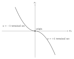
Figure 1:Switching curves for the minimum-time double integrator separate the terminal arcs associated with the two extreme controls.

Piecewise State Solution with One Switch¶

Suppose the control switches from -1 to +1 at $t=t_s$ .

For $0\leq t\leq t_s$ ,

\begin{aligned} x_2(t) &= x_{20}-t, \\ x_1(t) &= x_{10}+x_{20}t-\frac{1}{2}t^2. \end{aligned}

(53)

Define

\begin{aligned} x_{2s}&=x_2(t_s),\\ x_{1s}&=x_1(t_s). \end{aligned}

(54)

For $t_s\leq t\leq t_f$ ,

\begin{aligned} x_2(t) &= x_{2s}+(t-t_s), \\ x_1(t) &= x_{1s} + x_{2s}(t-t_s) + \frac{1}{2}(t-t_s)^2. \end{aligned}

(55)

For the reverse switch, from +1 to -1, the signs reverse:

\begin{aligned} x_2(t) &= x_{20}+t, \\ x_1(t) &= x_{10}+x_{20}t+\frac{1}{2}t^2, \qquad 0\leq t\leq t_s, \end{aligned}

(56)

followed by

\begin{aligned} x_2(t) &= x_{2s}-(t-t_s), \\ x_1(t) &= x_{1s} + x_{2s}(t-t_s) - \frac{1}{2}(t-t_s)^2. \end{aligned}

(57)

Computing the Switching Time¶

The switching time is determined by enforcing the terminal conditions:

x_1(t_f)=0, \qquad x_2(t_f)=0.

(58)

For a specified initial condition, one selects the switching sequence consistent with the phase-plane region and solves the resulting algebraic equations for $t_s$ and $t_f$ .

An equivalent geometric procedure is:

identify the constant-control parabola passing through the initial state;
determine its intersection with the appropriate terminal switching curve;
use that intersection as the switching point; and
compute the travel time along both arcs.

Why Minimum-Time Problems Favor Extreme Controls¶

If the control enters the dynamics linearly and the cost penalizes only elapsed time, reducing the magnitude of the control generally delays arrival.

Pontryagin’s Minimum Principle formalizes this intuition. Since the Hamiltonian is linear in $u$ , minimizing it over a bounded interval selects one of the endpoints.

Thus,

u^*(t)\in\{-1,+1\}

(59)

almost everywhere, except possibly at switching times or on singular arcs.

Higher-Order Integrator Systems¶

For the $r$ th-order integrator

x^{(r)}=u,

(60)

the costate components become higher-degree polynomials in time.

Therefore, the switching function can possess more zeros, and the optimal control can switch more than once.

The double integrator is especially simple because its switching function is affine in time and therefore has at most one zero.

Singular Arcs¶

A singular arc occurs when the switching function vanishes over a nonzero interval:

\sigma(t) = \frac{\partial H}{\partial u} = 0

(61)

for all $t$ in that interval.

On a singular arc, direct Hamiltonian minimization does not determine the control. One must differentiate the switching function until the control appears explicitly:

\sigma(t)=0, \quad \dot{\sigma}(t)=0, \quad \ddot{\sigma}(t)=0, \quad \ldots

(62)

The resulting conditions may produce a singular control law.

Singular arcs are common in:

chemical-process control;
bioreactor optimization;
aerospace trajectory optimization;
energy-management problems; and
systems with one-sided actuation.

One-Sided and Two-Sided Control¶

Mechanical systems often admit two-sided control:

-u_{\max}\leq u\leq u_{\max}.

(63)

Examples include positive and negative torque, force, or acceleration.

Many process systems instead admit one-sided control:

0\leq u\leq u_{\max}.

(64)

For example, material can be added to a reactor but may not be removable through the same control channel.

One-sided control can create asymmetric switching structures and often increases the likelihood of boundary and singular arcs.

Common Errors¶

Claiming that a free final time always implies $H^*=0$ .
Omitting the running-cost term 1 from a minimum-time Hamiltonian without explaining the adopted convention.
Applying $\partial H/\partial u=0$ to a Hamiltonian that is linear in a bounded control.
Ignoring the admissible control interval in Hamiltonian minimization.
Reversing the sign of the bang–bang law.
Assuming that $\lambda_2=0$ at an isolated switch implies a singular arc.
Treating a switching curve as a state trajectory valid for every control.
Forgetting continuity of the state at the switching time.

Summary¶

The main conclusions are:

Along an optimal trajectory,

\frac{\,\mathrm{d} H^*}{\,\mathrm{d} t} = \frac{\partial H}{\partial t}.

(65)

If the Hamiltonian has no explicit time dependence, it is constant.
If the final time is free and the endpoint terms have no explicit final-time dependence, then the constant Hamiltonian is zero.
The minimum-time double integrator has a Hamiltonian linear in the bounded control.
Stationarity does not determine the optimal control in this problem.
Pontryagin’s Minimum Principle yields

u^*=-\operatorname{sgn}(\lambda_2).

(66)

The switching function is affine in time and can cross zero at most once.
The optimal control is bang–bang with at most one switch.
Constant-control trajectories are parabolas in the phase plane.
Singular arcs require separate higher-order analysis but do not occur in the standard minimum-time double integrator.

Connection. Before treating more delicate switching behavior, it is useful to unify the common Bolza, Mayer, and Lagrange formulations and clarify minimum-time conventions.