The Goddard Rocket Problem and Singular Thrust
The Goddard rocket problem is a classical optimal-control problem in which a vertically ascending rocket uses a finite amount of fuel to maximize altitude. Despite its simple physical statement, the optimal thrust can contain a singular interval.
This section develops:
the one-dimensional rocket model;
the Mayer objective;
the Hamiltonian and costate equations;
the thrust switching function;
bang and singular thrust conditions;
differentiation of the singular condition;
bang–singular–coast structure; and
computational implications.
Problem Statement
Let:
be altitude;
be vertical velocity;
be mass;
be thrust;
be aerodynamic drag;
be gravitational acceleration; and
be effective exhaust velocity.
The objective is to maximize final altitude:
Using minimization notation,
The final time is free.
Dynamics
The one-dimensional ascent dynamics are
The thrust is bounded:
Typical initial conditions are
A fixed terminal mass is imposed:
The final altitude and final velocity are free.
Hamiltonian
Because the cost is in Mayer form and there is no running cost,
Therefore,
Group the thrust-dependent terms:
Hamiltonian Constancy
The Hamiltonian has no explicit time dependence:
Thus,
Since the final time is free and the terminal cost has no explicit dependence on ,
Therefore,
Costate Equations
The costate equations are
For altitude:
For velocity:
For mass:
Terminal Transversality Conditions
The terminal cost is
Since and are free,
The terminal mass is fixed, so is not prescribed directly.
Switching Function
The Hamiltonian is linear in thrust. Define
Pontryagin’s Minimum Principle gives
Thus:
gives maximum thrust;
gives zero thrust; and
is the singular candidate.
Equivalent Singular Condition
Multiply the switching function by :
Define
On a singular arc,
Since and , this condition is equivalent to .
First Derivative of the Singular Condition
Differentiate
Then
Substitute
where
This gives
Rearranging:
On the singular arc,
Hence the thrust-dependent term vanishes and
The first derivative still does not determine .
Second Derivative and Singular Thrust
Differentiate once more:
After substituting the state and costate dynamics, the second derivative has the general form
Therefore, the candidate singular thrust is
provided .
The explicit expressions depend on the selected drag law .
The candidate is admissible only if
A Common Drag Model
A frequently used model is
where
Then
These expressions simplify the costate and singular-thrust equations.
Expected Optimal Thrust Structure
The rocket must initially generate enough thrust to lift off, so the first arc is generally
A classical optimal structure is
This is a bang–singular–bang structure, where the final “bang” is the lower thrust bound.
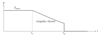
Figure 1:Expected bang–singular–bang thrust structure for the Goddard rocket problem.
Entry and Exit Conditions
The unknown singular entry time and exit time satisfy:
The state and costate must also be continuous:
These conditions, together with the endpoint conditions and integrated dynamics, determine the full multiphase solution.
Why Maximum Thrust Followed by Zero Is Not Always Optimal
A naive strategy is
This ignores the interaction among:
fuel consumption;
atmospheric drag;
changing mass;
velocity-dependent drag losses; and
the value of thrust at different altitudes.
The singular arc balances these effects. It can reduce drag losses while still using the available fuel effectively.
Numerical Formulation
A practical numerical solution can be posed as a multiphase problem:
Phase 1: .
Phase 2: and .
Phase 3: .
Unknowns include:
initial costates;
;
;
;
singular-arc state and costate values; and
possibly parameters of the drag model.
Continuity and endpoint conditions form the nonlinear residual system.
Verification Conditions
A computed solution should satisfy:
state dynamics;
costate dynamics;
thrust bounds;
Hamiltonian minimization;
;
terminal transversality;
on the singular arc;
continuity at and ; and
a generalized Legendre–Clebsch condition.
Common Errors
Using and assuming it directly gives thrust.
Ignoring the possibility over an interval.
Treating an isolated switching point as a singular arc.
Forgetting that final time is free.
Omitting the terminal Hamiltonian condition.
Using the wrong sign in the thrust switching law.
Assuming a candidate singular thrust is automatically admissible.
Failing to enforce continuity at the singular entry and exit points.
Summary
The Goddard rocket problem maximizes terminal altitude using bounded thrust.
The Hamiltonian is linear in thrust.
The switching function is
Negative gives maximum thrust and positive gives zero thrust.
defines a singular candidate.
The first derivative of the singular condition does not contain thrust.
The second derivative introduces thrust and yields a candidate singular law.
The optimal trajectory may have a maximum-thrust, singular-thrust, zero-thrust structure.
Entry and exit times must be solved as unknown events.
The problem illustrates how simple dynamics can produce highly nontrivial optimal controls.
Connection. Even an exact set of state–costate equations may be numerically ill conditioned, so the coupled Hamiltonian dynamics and shooting sensitivity deserve separate study.