Indirect Numerical Methods, Multiple Shooting, and Pontryagin’s Minimum Principle
Most optimal control problems cannot be solved analytically. Nonlinear dynamics, complicated endpoint conditions, control bounds, and long time horizons generally require numerical solution.
This section introduces two broad classes of numerical optimal control methods:
Indirect methods, which first derive necessary conditions and then solve the resulting boundary-value problem.
Direct methods, which discretize and optimize the original control problem directly.
The chapter focuses on indirect methods, especially:
Newton’s method for root finding;
single shooting;
multiple shooting;
continuity or checkpoint constraints;
parallel shooting; and
Pontryagin’s Minimum Principle for constrained controls.
Why Numerical Methods Are Necessary
Consider the general optimal control problem
subject to
Closed-form solutions are exceptional because:
the state equations are often nonlinear;
the costate equations are coupled to the state;
the endpoint conditions are split across two times;
the optimal control can switch between interior and boundary values; and
the resulting boundary-value problem may be unstable or highly sensitive.
Thus, computational methods are central to practical optimal control.
Indirect and Direct Optimization Methods
A finite-dimensional analogy
Suppose one wants to minimize a smooth scalar function
A necessary condition for an unconstrained local optimum is
Solving this condition is not itself an optimization problem. It is a root-finding problem:
The second derivative then classifies the critical point:
This is an indirect method: one derives necessary conditions and solves them.
By contrast, a direct method operates on itself and searches for a value that reduces the objective without first solving the stationarity equation exactly.
The Hamiltonian Boundary-Value Problem
For an unconstrained-control optimal control problem, the necessary conditions include
together with the endpoint constraints and transversality conditions.
Define the combined state–costate vector
After eliminating the control through stationarity when possible, the canonical equations can be written as
All endpoint and transversality conditions can be collected into a residual vector
Equations (9)–(10) form a two-point boundary-value problem.
The numerical task is to find unknown endpoint data such that integration of the differential equations produces zero boundary residual.
Newton’s Method for Root Finding
Suppose
is a system of nonlinear algebraic equations.
Let be the current iterate and write
A first-order Taylor expansion gives
Requiring the linearized residual to vanish yields
Therefore,
In computation, the Jacobian is not explicitly inverted. Instead, one solves the linear system
Convergence remarks
Newton’s method converges rapidly when:
the initial guess is sufficiently close to the root;
the residual is smooth;
the Jacobian is nonsingular; and
the Jacobian is computed accurately.
It may fail when the initial guess is poor or the Jacobian is ill-conditioned.
Single Shooting as a Root-Finding Problem
Suppose denotes the unknown initial data, often the initial costate:
For each guess :
form the complete initial condition;
integrate the canonical equations to ;
evaluate the terminal and transversality conditions; and
construct the shooting residual.
The residual may be written as
The shooting problem is
Newton’s method gives
Algorithm
Choose an initial guess .
Integrate the state–costate equations.
Evaluate the boundary residual .
Compute or approximate the shooting Jacobian.
Solve for the Newton correction.
Update the shooting variables.
Repeat until
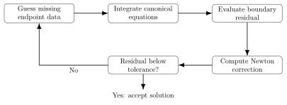
Figure 1:Newton shooting updates missing endpoint data until the boundary residual is below tolerance.
Sensitivity and the Shooting Jacobian
The shooting Jacobian measures the sensitivity of the boundary residual to the guessed endpoint variables:
It can be computed using:
finite differences;
variational or sensitivity equations;
automatic differentiation; or
complex-step differentiation when applicable.
For the parameterized initial-value problem
define the sensitivity matrix
Differentiating the dynamics gives
with
This matrix can then be used to construct the shooting Jacobian accurately.
Why Single Shooting Becomes Difficult
Single shooting integrates across the entire horizon. If the canonical dynamics contain growing modes, errors in the guessed endpoint data may grow exponentially.
The method becomes difficult when:
the time horizon is long;
the state–costate system is unstable;
the initial guess is poor;
the system contains multiple time scales;
the dynamics are strongly nonlinear; or
the boundary residual is poorly conditioned.
These limitations motivate multiple shooting.
Multiple Shooting
Partition the time interval:
Introduce an independent parameter at the beginning of each segment:
Starting from , integrate
over .
Let
denote the result of this integration at .
The independently introduced parameter at the next node is . Continuity requires
These are called:
matching constraints;
continuity constraints;
checkpoint constraints; or
defect constraints in a shooting context.
Why the next segment does not simply start from the previous result
If each segment simply starts from the endpoint produced by the previous segment, the procedure is identical to single shooting.
In multiple shooting, the initial value of each segment is an independent optimization or root-finding variable. The integrated endpoint and the next segment’s initial variable are allowed to differ during the iteration. Their equality is imposed only through the matching constraints.
This prevents unstable error growth from accumulating over the full horizon in a single integration.
Multiple-Shooting Residual
Collect all segment initial values into
The residual consists of:
the original endpoint conditions; and
all continuity conditions.
A general multiple-shooting residual is
The numerical problem is
Newton’s method or a related nonlinear root solver can then be applied.
Parallel Shooting Interpretation
Each segment integration depends only on its own initial parameter . Therefore, all segment integrations can be performed independently and, in principle, simultaneously.
This is why multiple shooting is also called parallel shooting.
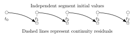
Figure 2:Multiple shooting uses independent segment initial values and enforces continuity through matching residuals.
Single Shooting Versus Multiple Shooting
| Feature | Single shooting | Multiple shooting |
|---|---|---|
| Number of variables | Small | Larger |
| Integration horizon | Entire interval | Short segments |
| Sensitivity to instability | High | Reduced |
| Memory requirement | Low | Higher |
| Parallelization | Limited | Natural |
| Implementation complexity | Lower | Higher |
| Initial-guess robustness | Often poor | Usually improved |
Multiple shooting trades additional variables and continuity constraints for improved numerical robustness.
Historical Computational Perspective
Indirect shooting was attractive in early computational optimal control because it introduced relatively few unknown variables.
If the state dimension is , then the state–costate vector has dimension . A basic shooting method may only need to solve for a subset of these endpoint values.
Multiple shooting introduces approximately additional variables per segment, increasing memory and algebraic problem size. Historically, this was a serious limitation.
Modern computers reduce this concern, but the tradeoff remains:
Practical MATLAB Workflow
A simple indirect-shooting implementation can be organized as follows:
Write a function for the state–costate dynamics.
Write a function that accepts the unknown shooting variables.
Construct the complete initial or terminal data.
Integrate using an ODE solver.
Evaluate the endpoint residual.
Pass the residual function to a nonlinear equation solver such as
fsolve.Verify the endpoint conditions after convergence.
A generic residual function has the conceptual form
function residual = shootingResidual(eta)
    p0 = constructInitialData(eta);
    [t,p] = ode45(@canonicalDynamics,[t0 tf],p0);
    pf = p(end,:)';
    residual = endpointConditions(p0,pf);
end
The converged numerical result should always be checked independently.
Transition to Constrained Controls
The stationarity condition
assumes that the optimal control lies in the interior of the allowable control set.
In practical systems, controls are usually bounded:
Examples include:
actuator-force limits;
torque limits;
steering-angle limits;
thrust limits;
angle-of-attack constraints;
voltage and current bounds; and
rate limits.
When the optimal control reaches a bound, the interior stationarity condition is not generally valid.
Pontryagin’s Minimum Principle
Suppose and are the optimal state and costate.
At each time, hold these optimal functions fixed and compare the Hamiltonian evaluated at an arbitrary admissible control with the Hamiltonian evaluated at the optimal control .
Optimality requires
for every admissible and almost every .
Equivalently,
Equation (39) is Pontryagin’s Minimum Principle under the minimum-Hamiltonian sign convention used here.
Minimum Principle Versus Stationarity
If the control set is unconstrained and the Hamiltonian is differentiable, the minimum principle often reduces to
If the control is bounded, the minimizer may occur at the boundary, so
can hold at the optimum.
Therefore:
Scalar Bounded-Control Illustration
Suppose
and the Hamiltonian depends linearly on the control:
The quantity
is the switching function.
Hamiltonian minimization gives
This structure motivates bang-bang and singular-control analysis.
Complete Indirect Optimality System
For a bounded-control problem, the indirect necessary conditions are:
together with:
endpoint constraints;
transversality conditions;
path constraints, when present; and
complementary or switching conditions, when needed.
The resulting system is generally a nonlinear two-point boundary-value problem solved by shooting, multiple shooting, or other numerical methods.
Common Errors
Treating the shooting residual as the original cost function.
Explicitly inverting a Newton Jacobian instead of solving a linear system.
Starting every multiple-shooting segment from the previous integrated endpoint.
Omitting the continuity constraints in multiple shooting.
Assuming remains valid at a control bound.
Minimizing the Hamiltonian over all real controls instead of the admissible set.
Confusing a necessary condition with a sufficient condition.
Accepting solver convergence without checking the endpoint residuals.
Summary
The main conclusions are:
Most optimal control problems require numerical solution.
Indirect methods solve the necessary conditions of optimality.
The optimality system becomes a root-finding problem coupled to differential equations.
Single shooting guesses missing endpoint data and iterates until the boundary conditions are satisfied.
Newton’s method provides a systematic shooting update.
Single shooting can be highly sensitive to unstable canonical dynamics.
Multiple shooting introduces independent segment initial values and continuity constraints.
Multiple shooting can be parallelized and is often more robust.
For constrained controls, Hamiltonian stationarity must be replaced by pointwise Hamiltonian minimization.
Pontryagin’s Minimum Principle is the appropriate general condition for selecting the optimal control.
Connection. The Hamiltonian formulation also yields conservation properties and switching rules, providing a direct route to minimum-time bang–bang control.