Coupled State–Costate Dynamics, Hamiltonian Matrices, and Shooting Instability

The first-order necessary conditions of optimal control form a coupled dynamical system. The state and costate cannot generally be solved independently because the optimal control depends on both.

This section develops that structure through a scalar quadratic optimal-control example and uses the result to explain why simple shooting can fail, even when:

the original dynamics are linear;
the optimality equations are solved analytically;
there is no numerical integration error; and
the initial costate guess is extremely accurate.

The main topics are:

coupled state–costate equations;
the costate as a sensitivity or dual variable;
a fixed-endpoint quadratic example;
eigenvalue and eigenvector analysis;
Hamiltonian matrix structure;
spectral symmetry of Hamiltonian systems;
propagation of shooting errors;
long-horizon instability; and
motivation for robust numerical optimal-control methods.

Canonical State–Costate Equations¶

Consider the optimal-control problem

\min_{\boldsymbol{u}(\cdot)} \left[ \Phi(\boldsymbol{x}(t_f),t_f) + \int_{t_0}^{t_f} L(\boldsymbol{x},\boldsymbol{u},t)\,\mathrm{d} t \right],

(1)

subject to

\dot{\boldsymbol{x}} = \boldsymbol{f}(\boldsymbol{x},\boldsymbol{u},t).

(2)

The Hamiltonian is

H(\boldsymbol{x},\boldsymbol{u},\boldsymbol{\lambda},t) = L(\boldsymbol{x},\boldsymbol{u},t) + \boldsymbol{\lambda}^{\mathsf{T}}\boldsymbol{f}(\boldsymbol{x},\boldsymbol{u},t).

(3)

The canonical equations are

\begin{aligned} \dot{\boldsymbol{x}} &= \left( \frac{\partial H}{\partial\boldsymbol{\lambda}} \right)^{\mathsf{T}}, \\ \dot{\boldsymbol{\lambda}} &= - \left( \frac{\partial H}{\partial\boldsymbol{x}} \right)^{\mathsf{T}}. \end{aligned}

(4)

Expanding the costate equation gives

\dot{\boldsymbol{\lambda}} = - \left[ \frac{\partial L}{\partial\boldsymbol{x}} + \boldsymbol{\lambda}^{\mathsf{T}} \frac{\partial\boldsymbol{f}}{\partial\boldsymbol{x}} \right]^{\mathsf{T}}.

(5)

Thus, the costate generally depends on:

the state;
the control;
the costate itself; and
possibly time.

Why the State and Costate Are Coupled¶

Suppose the pointwise optimality condition gives

\boldsymbol{u}^* = \boldsymbol{u}^*(\boldsymbol{x}^*,\boldsymbol{\lambda}^*,t).

(6)

Substitution into the state equation gives

\dot{\boldsymbol{x}}^* = \boldsymbol{f}\!\left( \boldsymbol{x}^*, \boldsymbol{u}^*(\boldsymbol{x}^*,\boldsymbol{\lambda}^*,t), t \right).

(7)

Therefore,

\dot{\boldsymbol{x}}^* = \boldsymbol{g}_x(\boldsymbol{x}^*,\boldsymbol{\lambda}^*,t).

(8)

Similarly,

\dot{\boldsymbol{\lambda}}^* = \boldsymbol{g}_\lambda(\boldsymbol{x}^*,\boldsymbol{\lambda}^*,t).

(9)

The combined optimality system is

\boxed{ \frac{\,\mathrm{d}}{\,\mathrm{d} t} \begin{bmatrix} \boldsymbol{x}^*\\ \boldsymbol{\lambda}^* \end{bmatrix} = \begin{bmatrix} \boldsymbol{g}_x(\boldsymbol{x}^*,\boldsymbol{\lambda}^*,t)\\ \boldsymbol{g}_\lambda(\boldsymbol{x}^*,\boldsymbol{\lambda}^*,t) \end{bmatrix}. }

(10)

The two systems must be solved simultaneously.

Interpretation of the Costate¶

The costate is a dual or adjoint variable associated with the state dynamics.

Conceptually, it measures the sensitivity of the optimal cost to a perturbation in the state.

A common interpretation is

\lambda_i(t) \sim \frac{\partial J^*}{\partial x_i(t)},

(11)

where $J^*$ denotes the optimal value function, subject to sign and formulation conventions.

If perturbing the state had no influence on the cost, then there would be no meaningful optimization pressure associated with that state direction.

The costate transmits this sensitivity through the optimality system and directly affects the optimal control.

A Scalar Quadratic Example¶

Consider

\boxed{ \min_{u(\cdot)} J = \frac{1}{2} \int_0^{t_f} \left( x^2+u^2 \right)\,\mathrm{d} t }

(12)

subject to

\dot{x} = x+u.

(13)

The time horizon $t_f$ is fixed, and the state is fixed at both endpoints:

\begin{aligned} x(0)&=x_0,\\ x(t_f)&=x_f. \end{aligned}

(14)

There is no terminal cost.

Hamiltonian and Optimal Control¶

The Hamiltonian is

H = \frac{1}{2} \left( x^2+u^2 \right) + \lambda(x+u).

(15)

The Hamiltonian is quadratic in $u$ , and the control is unconstrained. Therefore, the stationarity condition applies:

\frac{\partial H}{\partial u} = u+\lambda = 0.

(16)

Hence,

\boxed{ u^*=-\lambda^*. }

(17)

This formula explicitly demonstrates that the optimal control depends on the costate.

Coupled Optimality Dynamics¶

The state equation becomes

\dot{x}^* = x^*-\lambda^*.

(18)

The costate equation is

\begin{aligned} \dot{\lambda}^* &= -\frac{\partial H}{\partial x} \\ &= -\left(x^*+\lambda^*\right). \end{aligned}

(19)

Therefore,

\boxed{ \frac{\,\mathrm{d}}{\,\mathrm{d} t} \begin{bmatrix} x\\ \lambda \end{bmatrix} = \begin{bmatrix} 1 & -1\\ -1 & -1 \end{bmatrix} \begin{bmatrix} x\\ \lambda \end{bmatrix}. }

(20)

Define

\boldsymbol{p} = \begin{bmatrix} x\\ \lambda \end{bmatrix}, \qquad \boldsymbol{A} = \begin{bmatrix} 1 & -1\\ -1 & -1 \end{bmatrix}.

(21)

Then

\dot{\boldsymbol{p}} = \boldsymbol{A}\boldsymbol{p}.

(22)

Boundary Conditions¶

The state is fixed at both endpoints:

\begin{aligned} x(0)&=x_0,\\ x(t_f)&=x_f. \end{aligned}

(23)

Because both endpoint values of the state are fixed, the costate has no directly prescribed initial or final value.

Thus, the problem is a two-point boundary-value problem with:

one known state condition at $t=0$ ;
one known state condition at $t=t_f$ ; and
an unknown initial costate that must be selected correctly.

Eigenvalue Analysis¶

For

\dot{\boldsymbol{p}} = \boldsymbol{A}\boldsymbol{p},

(24)

the eigenvalues satisfy

\det(\mu\boldsymbol{I}-\boldsymbol{A})=0.

(25)

Here,

\mu\boldsymbol{I}-\boldsymbol{A} = \begin{bmatrix} \mu-1 & 1\\ 1 & \mu+1 \end{bmatrix}.

(26)

Therefore,

\begin{aligned} 0 &= (\mu-1)(\mu+1)-1 \\ &= \mu^2-2. \end{aligned}

(27)

Hence,

\boxed{ \mu_{1,2} = \pm\sqrt{2}. }

(28)

One eigenvalue is negative and the other is positive.

Thus, the state–costate dynamics contain:

one exponentially decaying mode in forward time; and
one exponentially growing mode in forward time.

Eigenvectors¶

For

\mu_1=-\sqrt{2},

(29)

an eigenvector satisfies

(\mu_1\boldsymbol{I}-\boldsymbol{A})\boldsymbol{v}_1=\boldsymbol{0}.

(30)

Choosing the second component equal to one gives

\boldsymbol{v}_1 = \begin{bmatrix} \dfrac{1}{1+\sqrt{2}}\\[2mm] 1 \end{bmatrix}.

(31)

For

\mu_2=+\sqrt{2},

(32)

one may choose

\boldsymbol{v}_2 = \begin{bmatrix} \dfrac{1}{1-\sqrt{2}}\\[2mm] 1 \end{bmatrix}.

(33)

The general solution is

\boxed{ \boldsymbol{p}(t) = C_1\boldsymbol{v}_1e^{-\sqrt{2}t} + C_2\boldsymbol{v}_2e^{+\sqrt{2}t}. }

(34)

Stable and Unstable Modes¶

In forward time:

e^{-\sqrt{2}t} \longrightarrow0,

(35)

whereas

e^{+\sqrt{2}t} \longrightarrow\infty.

(36)

In backward time, the roles reverse.

Therefore, integrating the full Hamiltonian system in either direction generally exposes one unstable mode.

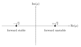
Figure 1:A Hamiltonian system exposes paired stable and unstable eigenvalues during forward integration.

Hamiltonian Matrix Structure¶

For a general canonical system,

\dot{\boldsymbol{p}} = \boldsymbol{g}(\boldsymbol{p}), \qquad \boldsymbol{p}= \begin{bmatrix} \boldsymbol{x}\\ \boldsymbol{\lambda} \end{bmatrix},

(37)

the Jacobian of the Hamiltonian vector field has the block form

\frac{\partial\boldsymbol{g}}{\partial\boldsymbol{p}} = \begin{bmatrix} H_{\lambda x} & H_{\lambda\lambda}\\ -H_{xx} & -H_{x\lambda} \end{bmatrix}.

(38)

This is a Hamiltonian matrix under the standard smoothness and symmetry assumptions on second derivatives.

A real matrix $\boldsymbol{A}$ is Hamiltonian if

\boldsymbol{A}^{\mathsf{T}}\boldsymbol{J}+\boldsymbol{J}\boldsymbol{A}=\boldsymbol{0},

(39)

where

\boldsymbol{J} = \begin{bmatrix} \boldsymbol{0} & \boldsymbol{I}\\ -\boldsymbol{I} & \boldsymbol{0} \end{bmatrix}.

(40)

Equivalently,

\boldsymbol{J}\boldsymbol{A}

(41)

is symmetric.

Spectral Symmetry¶

Hamiltonian matrices have a characteristic eigenvalue symmetry.

\mu

(42)

is an eigenvalue, then the spectrum also contains

-\mu.

(43)

For real matrices, complex conjugacy adds

\overline{\mu} \quad\text{and}\quad -\overline{\mu}.

(44)

Thus, a complex eigenvalue generally appears in a quartet:

\boxed{ \mu,\; -\mu,\; \overline{\mu},\; -\overline{\mu}. }

(45)

For a two-dimensional Hamiltonian system, only two eigenvalues exist. Therefore, a nonreal eigenvalue with nonzero real part would require four eigenvalues and cannot occur. The pair must instead lie:

symmetrically on the real axis; or
symmetrically on the imaginary axis.

In the present example, the pair is

\pm\sqrt{2}.

(46)

Simple Shooting Formulation¶

Suppose the unknown initial costate is guessed as

\lambda(0)=\bar{\lambda}_0.

(47)

Then

\begin{bmatrix} x(t)\\ \lambda(t) \end{bmatrix} = e^{\boldsymbol{A} t} \begin{bmatrix} x_0\\ \bar{\lambda}_0 \end{bmatrix}.

(48)

The shooting method adjusts $\bar{\lambda}_0$ until

x(t_f)=x_f.

(49)

Define the residual

R(\bar{\lambda}_0) = x(t_f;\bar{\lambda}_0)-x_f.

(50)

The desired initial costate satisfies

R(\lambda_0^*)=0.

(51)

Propagation of Initial-Costate Error¶

Let the exact initial costate be

\lambda_0^*.

(52)

Define the initial error

\delta\lambda_0 = \bar{\lambda}_0-\lambda_0^*.

(53)

The trajectory error is

\boldsymbol{e}(t) = \begin{bmatrix} x(t)-x^*(t)\\ \lambda(t)-\lambda^*(t) \end{bmatrix}.

(54)

Because the initial state is exact,

\boldsymbol{e}(0) = \begin{bmatrix} 0\\ \delta\lambda_0 \end{bmatrix}.

(55)

Therefore,

\boxed{ \boldsymbol{e}(t) = e^{\boldsymbol{A} t} \begin{bmatrix} 0\\ \delta\lambda_0 \end{bmatrix}. }

(56)

Using the eigendecomposition

\boldsymbol{A} = \boldsymbol{V}\boldsymbol{D}\boldsymbol{V}^{-1},

(57)

we have

e^{\boldsymbol{A} t} = \boldsymbol{V} \begin{bmatrix} e^{-\sqrt{2}t} & 0\\ 0 & e^{+\sqrt{2}t} \end{bmatrix} \boldsymbol{V}^{-1}.

(58)

Unless the initial error lies exactly in the stable eigenspace, it has a component that grows like

e^{+\sqrt{2}t}.

(59)

Long-Horizon Error Amplification¶

Suppose the initial costate error has magnitude

|\delta\lambda_0|=\varepsilon.

(60)

The unstable contribution at the final time behaves approximately as

\varepsilon e^{\sqrt{2}t_f}.

(61)

Thus, even a tiny initial error becomes large when $t_f$ is sufficiently long.

To maintain a fixed final error tolerance $\tau$ , the initial error must satisfy roughly

\varepsilon \lesssim \tau e^{-\sqrt{2}t_f}.

(62)

The required initial-costate accuracy therefore becomes exponentially severe with the horizon length.

Overflow Can Occur Without Integration Error¶

The instability is not caused only by numerical integration.

Even if

e^{\boldsymbol{A} t}

(63)

is evaluated analytically or exactly to machine precision, the unstable mode can exceed the largest representable floating-point number.

Thus, overflow may occur because of:

\text{dynamical instability},

(64)

not because of a low-order integration method.

A numerical integrator adds truncation and roundoff errors, which provide additional disturbances that can excite the unstable mode.

Why Backward Integration Does Not Solve the Problem¶

Forward integration contains the growing mode

e^{+\sqrt{2}t}.

(65)

One might attempt backward integration from $t_f$ . However, backward time reverses stability:

e^{-\sqrt{2}t}

(66)

becomes the growing mode under backward propagation.

Therefore, the Hamiltonian boundary-value problem is generally not converted into a well-conditioned initial-value problem merely by changing the direction of integration.

Shooting Jacobian Conditioning¶

For scalar shooting,

R(\lambda_0) = x(t_f;\lambda_0)-x_f.

(67)

Its derivative is

\frac{\,\mathrm{d} R}{\,\mathrm{d}\lambda_0} = \frac{\partial x(t_f)}{\partial\lambda_0}.

(68)

This sensitivity is a component of the state-transition matrix:

\frac{\partial\boldsymbol{p}(t_f)}{\partial\boldsymbol{p}(0)} = e^{\boldsymbol{A} t_f}.

(69)

Because this matrix contains exponentially large and small singular directions, the shooting Jacobian can become poorly scaled or ill-conditioned.

This makes Newton corrections sensitive to:

residual errors;
Jacobian approximation errors;
finite precision; and
the initial guess.

Stable and Unstable Manifold Interpretation¶

The exact optimal trajectory lies at the intersection of conditions imposed at opposite ends of the interval.

The initial endpoint conditions define a set of allowable initial points. The terminal conditions define a set of trajectories that arrive at the required terminal set.

The correct solution must lie on a special manifold that balances stable and unstable Hamiltonian modes.

A small error moves the trajectory away from this manifold, after which the unstable mode dominates.

Why Multiple Shooting Helps¶

Multiple shooting divides

\left[0,t_f\right]

(70)

into shorter intervals.

Instead of propagating one initial error over the full horizon, each segment propagates errors only over a shorter duration.

If the maximum segment length is $\Delta t$ , the local amplification behaves like

e^{\sqrt{2}\Delta t}

(71)

rather than

e^{\sqrt{2}t_f}.

(72)

Continuity constraints connect the segment solutions.

The method introduces more variables but improves conditioning.

Why Direct Methods Are Attractive¶

Direct methods avoid solving the continuous Hamiltonian boundary-value problem by shooting from one endpoint.

Instead, they discretize:

states;
controls;
dynamics;
path constraints; and
endpoint conditions.

The resulting nonlinear programming problem can exploit:

sparse linear algebra;
defect constraints;
scaling;
robust globalization strategies; and
simultaneous adjustment of the complete trajectory.

This does not eliminate all numerical difficulties, but it often avoids catastrophic initial-value sensitivity.

Practical Diagnostic Workflow¶

Before implementing simple shooting:

derive the coupled state–costate dynamics;
substitute the optimal control;
linearize around a representative trajectory;
inspect eigenvalues or finite-time growth;
estimate the amplification across the horizon;
inspect scaling and endpoint sensitivity;
test a short horizon first; and
use multiple shooting or direct methods if the system is strongly unstable.

Common Errors¶

Treating state and costate dynamics as decoupled.
Solving the costate first and substituting it afterward without justification.
Forgetting that the optimal control depends on the costate.
Assuming a linear original plant produces a stable Hamiltonian system.
Attributing every shooting failure to the ODE solver.
Assuming backward integration removes instability.
Ignoring exponential error amplification over long horizons.
Using simple shooting without inspecting the spectrum or sensitivities.
Confusing machine overflow with an algebraic error in the equations.
Simplifying the physical problem instead of selecting a suitable numerical method.

Summary¶

The main conclusions are:

State and costate equations form a coupled optimality system.
The costate represents the sensitivity of the cost to state perturbations.
In the quadratic example, the optimal control is $u^*=-\lambda^*$ .
The resulting Hamiltonian dynamics contain eigenvalues $\pm\sqrt{2}$ .
Hamiltonian spectra are symmetric about the real and imaginary axes.
One mode grows in forward time and another grows in backward time.
Initial-costate errors can grow exponentially across the horizon.
This failure can occur even with analytic propagation and no integration error.
Long-horizon simple shooting can exceed finite-precision capability.
Multiple shooting and direct methods provide more practical alternatives.

Connection. The final complication for the indirect framework is a constraint that acts continuously along the trajectory, creating active sets, multipliers, and constrained arcs.