Infinite-Horizon Linear Quadratic Regulation
This section continues the study of the linear quadratic optimal control problem. The main goals are:
to complete the interpretation of the finite-horizon Riccati solution;
to derive the infinite-horizon linear quadratic regulator;
to obtain the algebraic Riccati equation;
to explain the stabilizing Riccati solution;
to introduce the shooting method for two-point boundary-value problems; and
to show why shooting can become numerically unstable.
Finite-Horizon Linear Quadratic Optimal Control ¶ Consider the finite-horizon problem
min u ( ⋅ ) J = 1 2 x T ( t f ) S f x ( t f ) + 1 2 ∫ 0 t f [ x T Q x + u T R u ] d t , \min_{\boldsymbol{u}(\cdot)} J
=
\frac{1}{2}\boldsymbol{x}^{\mathsf{T}}(t_f)\boldsymbol{S}_f\boldsymbol{x}(t_f)
+
\frac{1}{2}\int_0^{t_f}
\left[
\boldsymbol{x}^{\mathsf{T}}\boldsymbol{Q}\boldsymbol{x}
+
\boldsymbol{u}^{\mathsf{T}}\boldsymbol{R}\boldsymbol{u}
\right]\,\mathrm{d} t, u ( ⋅ ) min J = 2 1 x T ( t f ) S f x ( t f ) + 2 1 ∫ 0 t f [ x T Q x + u T R u ] d t , subject to
x ˙ = A x + B u , x ( 0 ) = x 0 . \dot{\boldsymbol{x}}=\boldsymbol{A}\boldsymbol{x}+\boldsymbol{B}\boldsymbol{u},
\qquad
\boldsymbol{x}(0)=\boldsymbol{x}_0. x ˙ = A x + B u , x ( 0 ) = x 0 . The usual assumptions are
Q = Q T ⪰ 0 , R = R T ≻ 0 , \boldsymbol{Q}=\boldsymbol{Q}^{\mathsf{T}}\succeq 0,
\qquad
\boldsymbol{R}=\boldsymbol{R}^{\mathsf{T}}\succ 0, Q = Q T ⪰ 0 , R = R T ≻ 0 , together with controllability of ( A , B ) (\boldsymbol{A},\boldsymbol{B}) ( A , B )
The Hamiltonian is
H = 1 2 x T Q x + 1 2 u T R u + λ T ( A x + B u ) . H
=
\frac{1}{2}\boldsymbol{x}^{\mathsf{T}}\boldsymbol{Q}\boldsymbol{x}
+
\frac{1}{2}\boldsymbol{u}^{\mathsf{T}}\boldsymbol{R}\boldsymbol{u}
+
\boldsymbol{\lambda}^{\mathsf{T}}(\boldsymbol{A}\boldsymbol{x}+\boldsymbol{B}\boldsymbol{u}). H = 2 1 x T Q x + 2 1 u T R u + λ T ( A x + B u ) . Stationarity gives
∂ H ∂ u = R u + B T λ = 0 , \frac{\partial H}{\partial \boldsymbol{u}}
=
\boldsymbol{R}\boldsymbol{u}+\boldsymbol{B}^{\mathsf{T}}\boldsymbol{\lambda}
=
\boldsymbol{0}, ∂ u ∂ H = R u + B T λ = 0 , so
u ∗ = − R − 1 B T λ . \boldsymbol{u}^*
=
-\boldsymbol{R}^{-1}\boldsymbol{B}^{\mathsf{T}}\boldsymbol{\lambda}. u ∗ = − R − 1 B T λ . The costate equation is
λ ˙ = − Q x − A T λ . \dot{\boldsymbol{\lambda}}
=
-\boldsymbol{Q}\boldsymbol{x}-\boldsymbol{A}^{\mathsf{T}}\boldsymbol{\lambda}. λ ˙ = − Q x − A T λ . The terminal transversality condition is
λ ( t f ) = S f x ( t f ) . \boldsymbol{\lambda}(t_f)=\boldsymbol{S}_f\boldsymbol{x}(t_f). λ ( t f ) = S f x ( t f ) . Introduce
λ ( t ) = S ( t ) x ( t ) + β ( t ) . \boldsymbol{\lambda}(t)=\boldsymbol{S}(t)\boldsymbol{x}(t)+\boldsymbol{\beta}(t). λ ( t ) = S ( t ) x ( t ) + β ( t ) . After substitution into the state and costate equations, one obtains
x ˙ = ( A − B R − 1 B T S ) x − B R − 1 B T β , β ˙ = ( S B R − 1 B T − A T ) β + Γ ( S ) x , \begin{aligned}
\dot{\boldsymbol{x}}
&=
\left(
\boldsymbol{A}-\boldsymbol{B}\boldsymbol{R}^{-1}\boldsymbol{B}^{\mathsf{T}}\boldsymbol{S}
\right)\boldsymbol{x}
-
\boldsymbol{B}\boldsymbol{R}^{-1}\boldsymbol{B}^{\mathsf{T}}\boldsymbol{\beta},
\\
\dot{\boldsymbol{\beta}}
&=
\left(
\boldsymbol{S}\boldsymbol{B}\boldsymbol{R}^{-1}\boldsymbol{B}^{\mathsf{T}}-\boldsymbol{A}^{\mathsf{T}}
\right)\boldsymbol{\beta}
+
\boldsymbol{\Gamma}(\boldsymbol{S})\boldsymbol{x},
\end{aligned} x ˙ β ˙ = ( A − B R − 1 B T S ) x − B R − 1 B T β , = ( S B R − 1 B T − A T ) β + Γ ( S ) x , where
Γ ( S ) = − S ˙ − S A − A T S + S B R − 1 B T S − Q . \boldsymbol{\Gamma}(\boldsymbol{S})
=
-\dot{\boldsymbol{S}}
-\boldsymbol{S}\boldsymbol{A}
-\boldsymbol{A}^{\mathsf{T}}\boldsymbol{S}
+\boldsymbol{S}\boldsymbol{B}\boldsymbol{R}^{-1}\boldsymbol{B}^{\mathsf{T}}\boldsymbol{S}
-\boldsymbol{Q}. Γ ( S ) = − S ˙ − S A − A T S + S B R − 1 B T S − Q . Choose S \boldsymbol{S} S
Γ ( S ) = 0 . \boldsymbol{\Gamma}(\boldsymbol{S})=\boldsymbol{0}. Γ ( S ) = 0 . Then
S ˙ = − S A − A T S + S B R − 1 B T S − Q . \dot{\boldsymbol{S}}
=
-\boldsymbol{S}\boldsymbol{A}
-\boldsymbol{A}^{\mathsf{T}}\boldsymbol{S}
+\boldsymbol{S}\boldsymbol{B}\boldsymbol{R}^{-1}\boldsymbol{B}^{\mathsf{T}}\boldsymbol{S}
-\boldsymbol{Q}. S ˙ = − S A − A T S + S B R − 1 B T S − Q . Equation (13) Riccati differential equation .
Why the auxiliary term vanishes ¶ At t = t f t=t_f t = t f
λ ( t f ) = S ( t f ) x ( t f ) + β ( t f ) . \boldsymbol{\lambda}(t_f)=\boldsymbol{S}(t_f)\boldsymbol{x}(t_f)+\boldsymbol{\beta}(t_f). λ ( t f ) = S ( t f ) x ( t f ) + β ( t f ) . But the transversality condition requires
λ ( t f ) = S f x ( t f ) . \boldsymbol{\lambda}(t_f)=\boldsymbol{S}_f\boldsymbol{x}(t_f). λ ( t f ) = S f x ( t f ) . Choosing
S ( t f ) = S f \boldsymbol{S}(t_f)=\boldsymbol{S}_f S ( t f ) = S f gives
β ( t f ) = 0 . \boldsymbol{\beta}(t_f)=\boldsymbol{0}. β ( t f ) = 0 . Since
β ˙ = ( S B R − 1 B T − A T ) β \dot{\boldsymbol{\beta}}
=
\left(
\boldsymbol{S}\boldsymbol{B}\boldsymbol{R}^{-1}\boldsymbol{B}^{\mathsf{T}}-\boldsymbol{A}^{\mathsf{T}}
\right)\boldsymbol{\beta} β ˙ = ( S B R − 1 B T − A T ) β is a homogeneous linear differential equation, its solution can be written as
β ( t ) = Φ β ( t , t f ) β ( t f ) . \boldsymbol{\beta}(t)
=
\boldsymbol{\Phi}_{\beta}(t,t_f)\boldsymbol{\beta}(t_f). β ( t ) = Φ β ( t , t f ) β ( t f ) . Therefore,
β ( t ) ≡ 0 . \boxed{\boldsymbol{\beta}(t)\equiv \boldsymbol{0}.} β ( t ) ≡ 0 . Hence
λ ( t ) = S ( t ) x ( t ) . \boldsymbol{\lambda}(t)=\boldsymbol{S}(t)\boldsymbol{x}(t). λ ( t ) = S ( t ) x ( t ) . Finite-horizon optimal feedback law ¶ The optimal control becomes
u ∗ ( t ) = − R − 1 B T S ( t ) x ∗ ( t ) . \boxed{
\boldsymbol{u}^*(t)
=
-\boldsymbol{R}^{-1}\boldsymbol{B}^{\mathsf{T}}\boldsymbol{S}(t)\boldsymbol{x}^*(t).
} u ∗ ( t ) = − R − 1 B T S ( t ) x ∗ ( t ) . The corresponding closed-loop state equation is
x ˙ ∗ = [ A − B R − 1 B T S ( t ) ] x ∗ . \dot{\boldsymbol{x}}^*
=
\left[
\boldsymbol{A}-\boldsymbol{B}\boldsymbol{R}^{-1}\boldsymbol{B}^{\mathsf{T}}\boldsymbol{S}(t)
\right]\boldsymbol{x}^*. x ˙ ∗ = [ A − B R − 1 B T S ( t ) ] x ∗ . The finite-horizon solution procedure is therefore:
Integrate the Riccati differential equation backward from
S ( t f ) = S f . \boldsymbol{S}(t_f)=\boldsymbol{S}_f. S ( t f ) = S f . Use the resulting S ( t ) \boldsymbol{S}(t) S ( t )
K ( t ) = R − 1 B T S ( t ) . \boldsymbol{K}(t)=\boldsymbol{R}^{-1}\boldsymbol{B}^{\mathsf{T}}\boldsymbol{S}(t). K ( t ) = R − 1 B T S ( t ) . Integrate the state equation forward from x ( 0 ) = x 0 \boldsymbol{x}(0)=\boldsymbol{x}_0 x ( 0 ) = x 0
Recover
u ∗ ( t ) = − K ( t ) x ∗ ( t ) . \boldsymbol{u}^*(t)=-\boldsymbol{K}(t)\boldsymbol{x}^*(t). u ∗ ( t ) = − K ( t ) x ∗ ( t ) . Infinite-Horizon Linear Quadratic Regulator ¶ The infinite-horizon problem is
min u ( ⋅ ) J = 1 2 ∫ 0 ∞ [ x T Q x + u T R u ] d t , \min_{\boldsymbol{u}(\cdot)} J
=
\frac{1}{2}\int_0^\infty
\left[
\boldsymbol{x}^{\mathsf{T}}\boldsymbol{Q}\boldsymbol{x}
+
\boldsymbol{u}^{\mathsf{T}}\boldsymbol{R}\boldsymbol{u}
\right]\,\mathrm{d} t, u ( ⋅ ) min J = 2 1 ∫ 0 ∞ [ x T Q x + u T R u ] d t , subject to
x ˙ = A x + B u , x ( 0 ) = x 0 . \dot{\boldsymbol{x}}=\boldsymbol{A}\boldsymbol{x}+\boldsymbol{B}\boldsymbol{u},
\qquad
\boldsymbol{x}(0)=\boldsymbol{x}_0. x ˙ = A x + B u , x ( 0 ) = x 0 . Here A \boldsymbol{A} A B \boldsymbol{B} B Q \boldsymbol{Q} Q R \boldsymbol{R} R
This problem is the classical linear quadratic regulator , or LQR.
Finite horizon versus infinite horizon ¶ Feature Finite-horizon LQ problem Infinite-horizon LQR Time interval [ 0 , t f ] [0,t_f] [ 0 , t f ] [ 0 , ∞ ) [0,\infty) [ 0 , ∞ ) Terminal cost Usually present Usually absent Riccati equation Differential Algebraic Feedback gain Time varying Constant Computation Backward integration Matrix equation solve
Convergence Requirements on an Infinite Horizon ¶ For the cost
J = 1 2 ∫ 0 ∞ [ x T Q x + u T R u ] d t J
=
\frac{1}{2}\int_0^\infty
\left[
\boldsymbol{x}^{\mathsf{T}}\boldsymbol{Q}\boldsymbol{x}
+
\boldsymbol{u}^{\mathsf{T}}\boldsymbol{R}\boldsymbol{u}
\right]\,\mathrm{d} t J = 2 1 ∫ 0 ∞ [ x T Q x + u T R u ] d t to remain finite, the integrand must approach zero:
lim t → ∞ [ x T Q x + u T R u ] = 0. \lim_{t\to\infty}
\left[
\boldsymbol{x}^{\mathsf{T}}\boldsymbol{Q}\boldsymbol{x}
+
\boldsymbol{u}^{\mathsf{T}}\boldsymbol{R}\boldsymbol{u}
\right]
=
0. t → ∞ lim [ x T Q x + u T R u ] = 0. Because
Q ⪰ 0 , R ≻ 0 , \boldsymbol{Q}\succeq 0,
\qquad
\boldsymbol{R}\succ 0, Q ⪰ 0 , R ≻ 0 , the two nonnegative terms cannot cancel one another. Therefore,
lim t → ∞ x T Q x = 0 , lim t → ∞ u T R u = 0. \begin{aligned}
\lim_{t\to\infty}\boldsymbol{x}^{\mathsf{T}}\boldsymbol{Q}\boldsymbol{x} &= 0,
\\
\lim_{t\to\infty}\boldsymbol{u}^{\mathsf{T}}\boldsymbol{R}\boldsymbol{u} &= 0.
\end{aligned} t → ∞ lim x T Q x t → ∞ lim u T R u = 0 , = 0. Under the standard controllability and observability assumptions, this implies
x ∗ ( t ) → 0 , u ∗ ( t ) → 0 as t → ∞ . \boldsymbol{x}^*(t)\to \boldsymbol{0},
\qquad
\boldsymbol{u}^*(t)\to \boldsymbol{0}
\qquad
\text{as }t\to\infty. x ∗ ( t ) → 0 , u ∗ ( t ) → 0 as t → ∞. Since
λ = S x , \boldsymbol{\lambda}=\boldsymbol{S}\boldsymbol{x}, λ = S x , the optimal costate also satisfies
λ ∗ ( t ) → 0 . \boldsymbol{\lambda}^*(t)\to \boldsymbol{0}. λ ∗ ( t ) → 0 . The Algebraic Riccati Equation ¶ For the infinite-horizon, time-invariant problem, the steady-state Riccati matrix is constant. Hence
S ˙ = 0 . \dot{\boldsymbol{S}}=\boldsymbol{0}. S ˙ = 0 . Substituting this into the Riccati differential equation gives
− S A − A T S + S B R − 1 B T S − Q = 0 . -\boldsymbol{S}\boldsymbol{A}
-\boldsymbol{A}^{\mathsf{T}}\boldsymbol{S}
+\boldsymbol{S}\boldsymbol{B}\boldsymbol{R}^{-1}\boldsymbol{B}^{\mathsf{T}}\boldsymbol{S}
-\boldsymbol{Q}
=
\boldsymbol{0}. − S A − A T S + S B R − 1 B T S − Q = 0 . Equivalently,
A T S + S A − S B R − 1 B T S + Q = 0 . \boxed{
\boldsymbol{A}^{\mathsf{T}}\boldsymbol{S}
+
\boldsymbol{S}\boldsymbol{A}
-
\boldsymbol{S}\boldsymbol{B}\boldsymbol{R}^{-1}\boldsymbol{B}^{\mathsf{T}}\boldsymbol{S}
+
\boldsymbol{Q}
=
\boldsymbol{0}.
} A T S + S A − S B R − 1 B T S + Q = 0 . Equation (38) algebraic Riccati equation .
The infinite-horizon feedback law is
u ∗ = − K x ∗ , K = R − 1 B T S . \boxed{
\boldsymbol{u}^*
=
-\boldsymbol{K}\boldsymbol{x}^*,
\qquad
\boldsymbol{K}=\boldsymbol{R}^{-1}\boldsymbol{B}^{\mathsf{T}}\boldsymbol{S}.
} u ∗ = − K x ∗ , K = R − 1 B T S . The closed-loop dynamics are
x ˙ ∗ = ( A − B K ) x ∗ . \dot{\boldsymbol{x}}^*
=
(\boldsymbol{A}-\boldsymbol{B}\boldsymbol{K})\boldsymbol{x}^*. x ˙ ∗ = ( A − B K ) x ∗ . The Stabilizing Riccati Solution ¶ The algebraic Riccati equation is nonlinear and quadratic in S \boldsymbol{S} S
symmetric;
positive semidefinite or positive definite under stronger assumptions; and
stabilizing.
The stabilizing solution satisfies
Re [ λ i ( A − B R − 1 B T S ) ] < 0 \operatorname{Re}
\left[
\lambda_i(\boldsymbol{A}-\boldsymbol{B}\boldsymbol{R}^{-1}\boldsymbol{B}^{\mathsf{T}}\boldsymbol{S})
\right]
<0 Re [ λ i ( A − B R − 1 B T S ) ] < 0 for every closed-loop eigenvalue.
Thus,
x ∗ ( t ) → 0 as t → ∞ . \boldsymbol{x}^*(t)\to\boldsymbol{0}
\qquad
\text{as }t\to\infty. x ∗ ( t ) → 0 as t → ∞. For moderate state dimension, the algebraic Riccati equation is solved efficiently using standard numerical linear algebra routines.
For large-scale systems, however, direct solution becomes expensive because S ∈ R n × n \boldsymbol{S}\in\mathbb{R}^{n\times n} S ∈ R n × n A \boldsymbol{A} A B \boldsymbol{B} B
This issue appears frequently after spatial discretization of distributed-parameter systems such as:
A spatial discretization can create hundreds or thousands of states, making the Riccati equation itself a large-scale computational problem.
Return to the State–Costate Boundary-Value Problem ¶ Before the Riccati transformation, the finite-horizon optimality system is
d d t [ x λ ] = [ A − B R − 1 B T − Q − A T ] [ x λ ] . \frac{\,\mathrm{d}}{\,\mathrm{d} t}
\begin{bmatrix}
\boldsymbol{x}\\
\boldsymbol{\lambda}
\end{bmatrix}
=
\begin{bmatrix}
\boldsymbol{A} & -\boldsymbol{B}\boldsymbol{R}^{-1}\boldsymbol{B}^{\mathsf{T}}\\
-\boldsymbol{Q} & -\boldsymbol{A}^{\mathsf{T}}
\end{bmatrix}
\begin{bmatrix}
\boldsymbol{x}\\
\boldsymbol{\lambda}
\end{bmatrix}. d t d [ x λ ] = [ A − Q − B R − 1 B T − A T ] [ x λ ] . The boundary conditions are split between the two endpoints:
x ( 0 ) = x 0 , λ ( t f ) = S f x ( t f ) . \boldsymbol{x}(0)=\boldsymbol{x}_0,
\qquad
\boldsymbol{\lambda}(t_f)=\boldsymbol{S}_f\boldsymbol{x}(t_f). x ( 0 ) = x 0 , λ ( t f ) = S f x ( t f ) . This is a two-point boundary-value problem. The initial state is known, but the initial costate is unknown. At the terminal time, the state is unknown and only a relation between state and costate is available.
If
Φ ( t , τ ) \boldsymbol{\Phi}(t,\tau) Φ ( t , τ ) denotes the state-transition matrix of (43)
[ x ( t ) λ ( t ) ] = Φ ( t , τ ) [ x ( τ ) λ ( τ ) ] . \begin{bmatrix}
\boldsymbol{x}(t)\\
\boldsymbol{\lambda}(t)
\end{bmatrix}
=
\boldsymbol{\Phi}(t,\tau)
\begin{bmatrix}
\boldsymbol{x}(\tau)\\
\boldsymbol{\lambda}(\tau)
\end{bmatrix}. [ x ( t ) λ ( t ) ] = Φ ( t , τ ) [ x ( τ ) λ ( τ ) ] . The transition matrix alone does not remove the missing-boundary-condition problem.
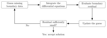
The Shooting Method ¶ The shooting method converts a boundary-value problem into an iterative sequence of initial-value problems.
Suppose the initial costate is unknown. Define a guess
λ ( 0 ) = η . \boldsymbol{\lambda}(0)=\boldsymbol{\eta}. λ ( 0 ) = η . For any chosen η \boldsymbol{\eta} η t f t_f t f
r ( η ) = λ ( t f ; η ) − S f x ( t f ; η ) . \boldsymbol{r}(\boldsymbol{\eta})
=
\boldsymbol{\lambda}(t_f;\boldsymbol{\eta})
-
\boldsymbol{S}_f\boldsymbol{x}(t_f;\boldsymbol{\eta}). r ( η ) = λ ( t f ; η ) − S f x ( t f ; η ) . The correct initial costate satisfies
r ( η ∗ ) = 0 . \boxed{
\boldsymbol{r}(\boldsymbol{\eta}^*)=\boldsymbol{0}.
} r ( η ∗ ) = 0 . The shooting method therefore solves the nonlinear root-finding problem
η ∗ = arg { r ( η ) = 0 } . \boldsymbol{\eta}^*
=
\arg\left\{
\boldsymbol{r}(\boldsymbol{\eta})=\boldsymbol{0}
\right\}. η ∗ = arg { r ( η ) = 0 } . A Newton update takes the form
η k + 1 = η k − [ ∂ r ∂ η ] − 1 r ( η k ) . \boldsymbol{\eta}_{k+1}
=
\boldsymbol{\eta}_k
-
\left[
\frac{\partial \boldsymbol{r}}{\partial \boldsymbol{\eta}}
\right]^{-1}
\boldsymbol{r}(\boldsymbol{\eta}_k). η k + 1 = η k − [ ∂ η ∂ r ] − 1 r ( η k ) . Backward shooting ¶ One may instead guess the unknown terminal state:
x ( t f ) = ζ , \boldsymbol{x}(t_f)=\boldsymbol{\zeta}, x ( t f ) = ζ , construct
λ ( t f ) = S f ζ , \boldsymbol{\lambda}(t_f)=\boldsymbol{S}_f\boldsymbol{\zeta}, λ ( t f ) = S f ζ , and integrate backward. The residual is then
r ( ζ ) = x ( 0 ; ζ ) − x 0 . \boldsymbol{r}(\boldsymbol{\zeta})
=
\boldsymbol{x}(0;\boldsymbol{\zeta})-\boldsymbol{x}_0. r ( ζ ) = x ( 0 ; ζ ) − x 0 . Both approaches seek a boundary guess that causes the integrated trajectory to hit the boundary conditions at the opposite endpoint.
Figure 1: Shooting iterates between a boundary-data guess, trajectory integration, residual evaluation, and guess update.
Why Shooting Can Be Numerically Unstable ¶ Consider the scalar problem
J = 1 2 s f x 2 ( t f ) + 1 2 ∫ 0 t f ( q x 2 + r u 2 ) d t , J
=
\frac{1}{2}s_f x^2(t_f)
+
\frac{1}{2}\int_0^{t_f}
\left(
q x^2+r u^2
\right)\,\mathrm{d} t, J = 2 1 s f x 2 ( t f ) + 2 1 ∫ 0 t f ( q x 2 + r u 2 ) d t , subject to
x ˙ = a x + b u , x ( 0 ) = x 0 , \dot{x}=ax+bu,
\qquad
x(0)=x_0, x ˙ = a x + b u , x ( 0 ) = x 0 , where
q > 0 , r > 0 , b ≠ 0. q>0,
\qquad
r>0,
\qquad
b\neq 0. q > 0 , r > 0 , b = 0. The state–costate system is
d d t [ x λ ] = [ a − b 2 / r − q − a ] ⏟ F [ x λ ] . \frac{\,\mathrm{d}}{\,\mathrm{d} t}
\begin{bmatrix}
x\\
\lambda
\end{bmatrix}
=
\underbrace{
\begin{bmatrix}
a & -b^2/r\\
-q & -a
\end{bmatrix}
}_{\boldsymbol{F}}
\begin{bmatrix}
x\\
\lambda
\end{bmatrix}. d t d [ x λ ] = F [ a − q − b 2 / r − a ] [ x λ ] . The characteristic equation is
det ( μ I − F ) = 0. \det(\mu\boldsymbol{I}-\boldsymbol{F})=0. det ( μ I − F ) = 0. Thus,
det [ μ − a b 2 / r q μ + a ] = 0 , \det
\begin{bmatrix}
\mu-a & b^2/r\\
q & \mu+a
\end{bmatrix}
=0, det [ μ − a q b 2 / r μ + a ] = 0 , which gives
μ 2 − a 2 − b 2 q r = 0. \mu^2-a^2-\frac{b^2q}{r}=0. μ 2 − a 2 − r b 2 q = 0. Therefore,
μ 1 , 2 = ± a 2 + b 2 q r . \boxed{
\mu_{1,2}
=
\pm
\sqrt{
a^2+\frac{b^2q}{r}
}.
} μ 1 , 2 = ± a 2 + r b 2 q . The eigenvalues are real, nonzero, and symmetric about the origin.
Let
μ = a 2 + b 2 q r > 0. \mu
=
\sqrt{
a^2+\frac{b^2q}{r}
}>0. μ = a 2 + r b 2 q > 0. Then the general solution contains one growing and one decaying mode:
p ( t ) = c 1 e μ t v 1 + c 2 e − μ t v 2 . \boldsymbol{p}(t)
=
c_1e^{\mu t}\boldsymbol{v}_1
+
c_2e^{-\mu t}\boldsymbol{v}_2. p ( t ) = c 1 e μ t v 1 + c 2 e − μ t v 2 . Forward integration ¶ During forward integration, the mode
grows exponentially. Any small component of the initial-guess error along this mode is amplified.
Backward integration ¶ During backward integration, the mode that decays in forward time becomes unstable. Thus, the term associated with
grows when time is traversed backward.
Therefore, the state–costate system is unstable in either integration direction.
Consequences for Numerical Optimal Control ¶ Shooting methods may fail or become poorly conditioned when:
the time horizon is long;
the system contains strongly unstable modes;
the initial guess is not close to the solution;
the costate dynamics are highly sensitive;
the dynamics are nonlinear; or
the integrator introduces accumulated numerical error.
These limitations motivate more robust methods such as:
Summary ¶ The major conclusions are:
In the finite-horizon LQ problem, the costate can be written as
λ ( t ) = S ( t ) x ( t ) . \boldsymbol{\lambda}(t)=\boldsymbol{S}(t)\boldsymbol{x}(t). λ ( t ) = S ( t ) x ( t ) . The matrix S ( t ) \boldsymbol{S}(t) S ( t )
S ( t f ) = S f . \boldsymbol{S}(t_f)=\boldsymbol{S}_f. S ( t f ) = S f . The finite-horizon feedback gain is time varying.
The infinite-horizon LQR produces the algebraic Riccati equation.
The relevant algebraic Riccati solution is the stabilizing symmetric solution.
The resulting LQR feedback gain is constant.
A two-point boundary-value problem can be solved iteratively using shooting.
Shooting may become numerically unstable because the Hamiltonian state–costate system contains both growing and decaying modes.
Connection. LQR is unusually tractable; for general nonlinear problems the same necessary conditions form a boundary-value problem that must be solved numerically.