Model Predictive Control

Model predictive control bridges optimal control and practical feedback. At each time step, MPC solves a finite-horizon problem using the current state estimate and possibly short-term forecasts. It applies only the first action, advances one step, and solves again.

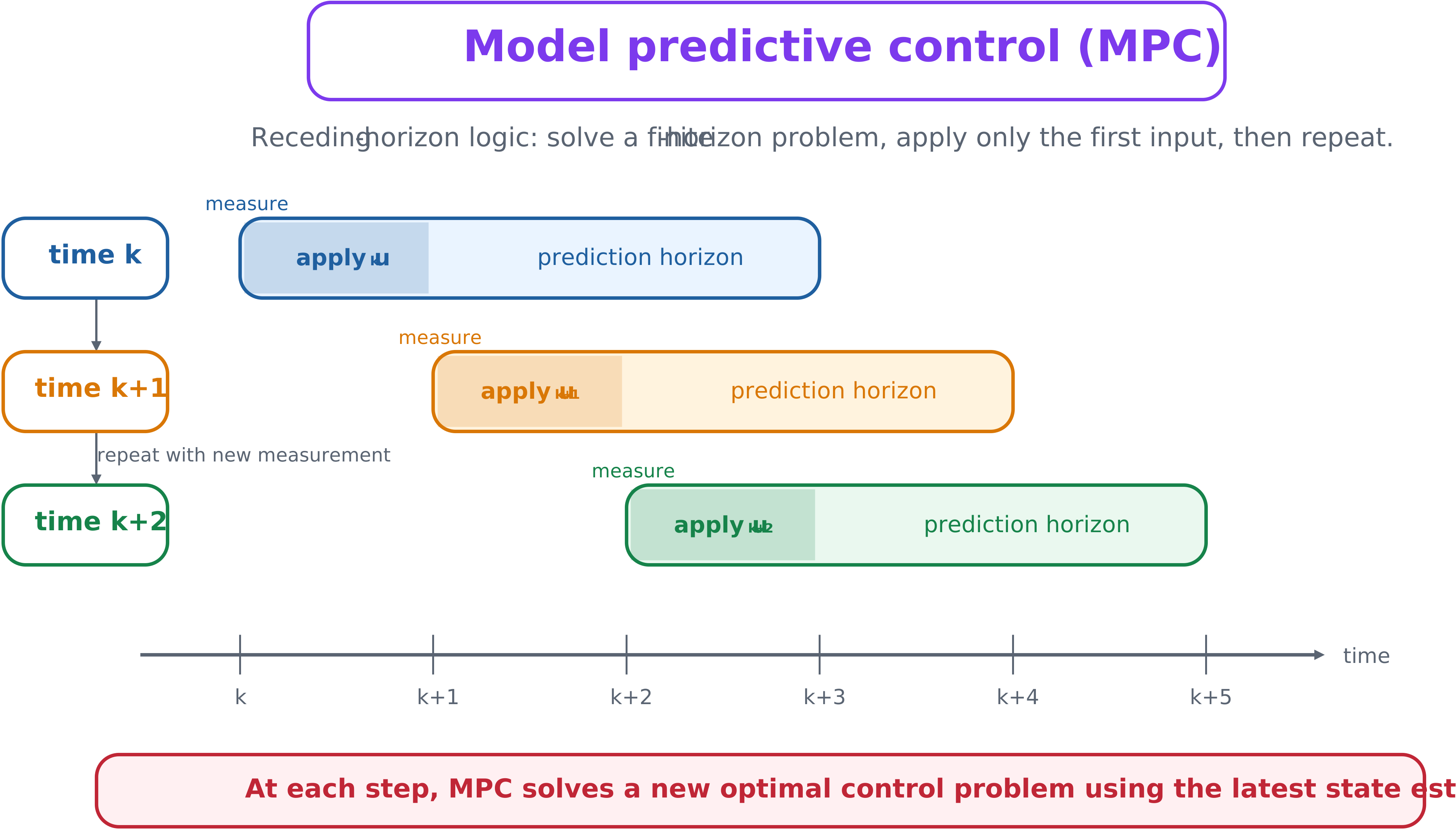
The receding-horizon strategy repeatedly updates a local open-loop plan.

Why MPC is feedback¶

Each internal optimization is open loop, but the overall controller is closed loop because every new solve uses updated measurements or estimates.

At time $k$:

1. measure or estimate $\mathbf{x}_k$;

2. solve a finite-horizon optimal-control problem;

3. obtain $\mathbf{u}_k,\ldots,\mathbf{u}_{k+N-1}$;

4. apply only $\mathbf{u}_k$; and

5. advance and repeat.

Advantages¶

• Incorporates a predictive model directly.

• Handles multivariable systems naturally.

• Enforces state and input constraints.

• Updates from measurements, creating feedback.

• Can use preview and short-term forecasts.

Limitations¶

• Requires online optimization.

• Depends on model quality.

• Is sensitive to horizon length and discretization.

• Can be difficult to execute in real time for fast or large systems.

MPC in CCD¶

Plant design may be optimized with MPC prediction horizon, control horizon, weighting matrices, and estimator settings. This gives a more implementable closed-loop formulation than pure OLOC while retaining optimization-based constraint handling.

Prediction horizon as an information-availability dial¶

A 2026 vehicle-suspension study frames the MPC prediction horizon explicitly as a tunable “information availability” setting rather than a fixed implementation detail. Two hyperparameters govern how much information the controller effectively has: the prediction horizon $p$ (an integer number of discrete steps) and the control sampling time $T_s$, which together give a prediction horizon length in time of $T_p=pT_s$. A control horizon $m\leq p$ specifies how many of those steps the control signal is allowed to vary over; setting $m=p$ keeps comparisons fair as $p$ is increased. With a very short horizon, MPC behaves close to a simple feedback controller; as $p$ grows, together with a finer model and more frequent updates, MPC approaches the accuracy of OLOC—though, unlike OLOC, it still incorporates no explicit knowledge of the past.

This makes $p$ (and $T_s$) genuine control-design variables that can themselves be optimized inside a nested CCD architecture: an outer loop uses the covariance matrix adaptation evolution strategy (CMA-ES)—a gradient-free, stochastic, population-based global optimizer well suited to nonconvex, nonseparable, and noisy objectives—to choose plant design variables, while an inner loop evaluates each candidate plant by running a full closed-loop MPC (or OLOC) simulation and returning the resulting objective value.

State estimation with a hybrid Kalman filter¶

MPC needs a state estimate at every sampling instant, but the plant is naturally modeled with continuous-time dynamics while sensor data arrives at discrete instants. A hybrid Kalman filter matches this mismatch: it propagates a continuous-time model,

forward between measurements, and performs a discrete-time update using

whenever a new measurement $\mathbf{y}_k$ arrives. The updated state estimate initializes the next MPC solve, and the controller never sees the true state directly—only the sensed outputs $\mathbf{y}_k$. Because the Kalman gain and error covariance in this linear setting are not themselves functions of the measured data, they can be computed offline and, after an initial transient, replaced by a constant steady-state gain instead of the full time-varying gain, substantially reducing online computation with little effect on estimation accuracy.

Activity 6.5: Nested Plant--MPC Co-Design¶