From OLOC to Implementable Control
A productive development path is:
solve an ideal OLOC problem;
study its control patterns and performance;
choose a realizable controller structure that captures the important behavior; and
co-design the plant with that implementable controller.
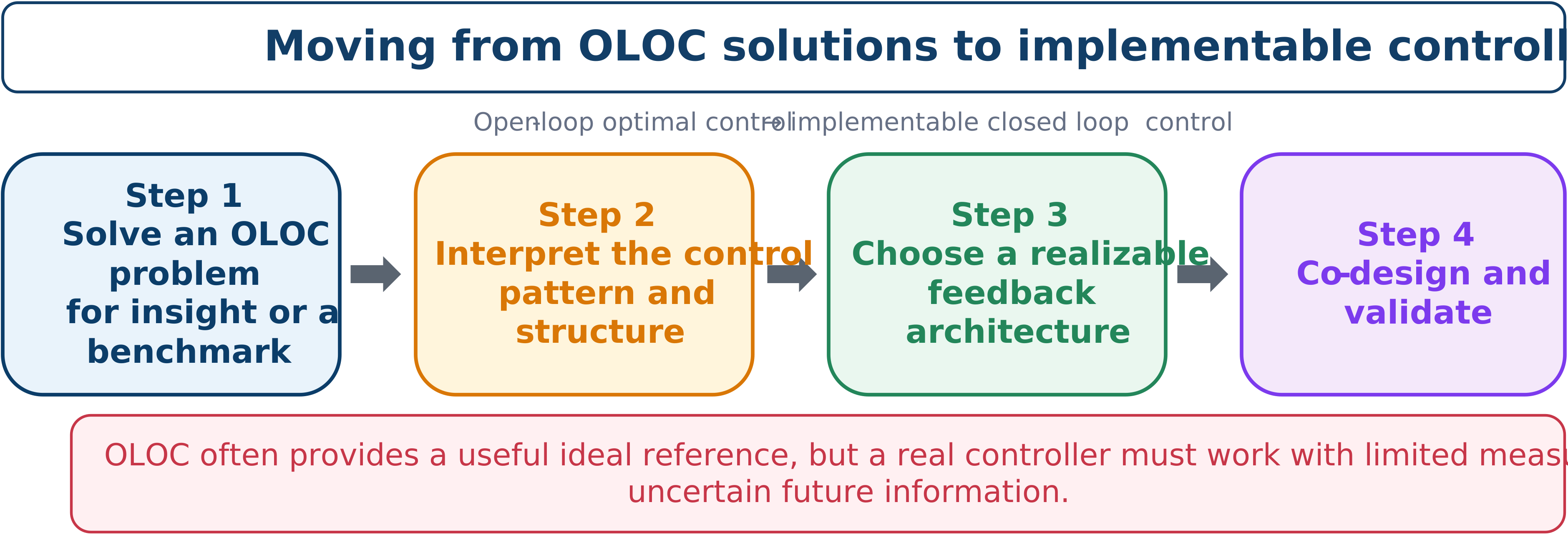
An ideal trajectory can guide—but should not be confused with—the final controller.
What OLOC can teach us
An optimal trajectory can reveal:
when control action should be active;
whether it behaves like stiffness, damping, or phase lead;
required control bandwidth and authority; and
which physical plant properties are most valuable.
Typical transitions
OLOC PID or gain-scheduled feedback.
OLOC LQR or state feedback.
OLOC MPC.
OLOC a rule-based controller informed by optimal behavior.
OLOC a parameterized policy fitted to optimal trajectories.
OLOC remains valuable because it supplies a best-case reference, explains ideal behavior, benchmarks practical controllers, and helps separate plant limitations from controller limitations. It is often best treated as an intermediate design-analysis tool.
A three-stage design framework
One way to operationalize the OLOC-to-implementable-control transition is a three-stage process developed for dynamic-system architecture design:
Stage 1 — plant architecture design, co-designed with OLC. The physical architecture and its design variables are optimized together with an unrestricted control trajectory . No actuator or control-architecture assumptions are made, so this stage searches the broadest design space and produces a system-optimal benchmark plant.
Stage 2 — controller architecture design, co-designed with CLC. A specific, implementable control architecture (for example, full-state feedback with optimized gains) is selected, and the plant is re-optimized jointly with that controller’s finite-dimensional parameter vector.
Stage 3 — digital controller design. The continuous-time control law produced in Stage 2 is realized as a digital controller, addressing sampling, discretization, and computation.
Mechanical engineers typically own Stage 1, while control engineers own Stages 2 and 3. Iteration between stages—and revision of a stage’s own formulation—is expected as insights from later stages feed back into earlier ones.
A worked progression: semi-active suspension
A trailing-arm quarter-car suspension study shows how performance degrades, in a controlled and explainable way, as each stage adds a layer of realism. Each row below is informed by the solution of the previous one:
| Problem | Control representation | Change | |
|---|---|---|---|
| P0 — passive | fixed linear damping, no active or semi-active control | an idealized passive benchmark that cannot actually be realized, because underlying geometric nonlinearities keep true passive damping nonlinear | |
| P1 — active OLC | unrestricted actuator force (Stage 1) | benchmark: best achievable performance with no actuator or architecture restriction | |
| P2 — semi-active OLC, ideal damper | force restricted to always dissipate energy, , | about worse than P1 | |
| P3 — semi-active OLC, realistic MR-damper model | current-to-force map identified from a physical damper | about worse than P2 | |
| P4 — semi-active CLC, full-state feedback (Stage 2) | optimized feedback gains acting on measured/estimated states, damper current as the physical output, | about worse than P3; about worse than the P1 benchmark |
The P2 solution was used to select and size an actual component: a Lord 8041-1 magnetorheological (MR) damper, with a continuous current operating range of 0-1 A and a maximum stroke of 74 mm. That damper’s hysteretic, current-dependent force-velocity behavior was characterized in the laboratory to build the P3 surrogate model, . In P4, all states were assumed measurable—mass accelerations from accelerometers, relative displacements from linear encoders, and velocities obtained by integrating the acceleration signals—and the feedback gains were optimized subject to the damper’s saturation limits. No single step in P1 P4 involved a design mistake: each one simply removed an assumption (unlimited actuator authority, an idealized semi-active component, or unlimited state/future information) that a real system cannot provide, and the resulting performance gap is the accumulated cost of implementability.
Activity 6.6: Converting an OLOC Trajectory into TVLQR Feedback
Activity 6.6: Converting an OLOC Trajectory into TVLQR Feedback
Consider a torque-controlled pendulum. Let denote the upright position and the downward position.
The dynamics are
Use
and
The boundary conditions are
Minimize
Solve the swing-up OLOC problem using GPOPS-II or Dymos.
Denote the optimal trajectory by
Linearize the dynamics along the optimal trajectory and show that
Solve the time-varying Riccati equation
with terminal condition
Implement the trajectory-tracking controller
Compare pure open-loop implementation and TVLQR feedback for the perturbed initial conditions
Repeat with
and additive measurement noise.
Report
Determine the largest initial perturbation for which the TVLQR controller successfully reaches the upright neighborhood
Explain why the OLOC trajectory remains valuable even though it is not robust enough for direct implementation.