1.2 The Physical Plant and Controller as a Single System

The closed-loop model is the design object¶

Consider a parameterized linear plant

\dot{x}(t)=A(p)x(t)+B(p)u(t)+E(p)d(t), \qquad y(t)=C(p)x(t),

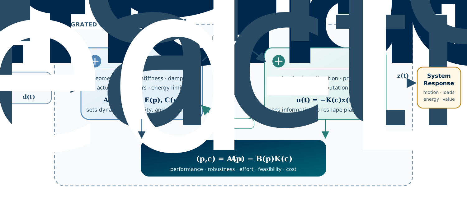
where $p$ contains physical decisions such as geometry, stiffness, mass distribution, motor constants, or actuator placement. With state feedback $u(t)=-K(c)x(t)$ , where $c$ denotes controller parameters, the closed-loop dynamics are

\dot{x}(t)=\left[A(p)-B(p)K(c)\right]x(t)+E(p)d(t).

The system poles, transient response, disturbance amplification, and control effort are properties of $A(p)-B(p)K(c)$ —not of $A$ , $B$ , or $K$ in isolation. Physical variables may alter both natural dynamics $A(p)$ and control authority $B(p)$ . Controller variables then reshape how those physical properties appear in operation.

Design effects travel in both directions between plant and controller.

Physical meaning of the coupling¶

The integrated view reveals recurring mechanisms:

Physical decision	Control consequence	System consequence
Lower structural mass	Faster motion, often more flexible modes	Efficiency may improve while robustness margins shrink
Larger actuator	More force and bandwidth	Better regulation but higher mass, heat, and cost
Higher gear ratio	More output torque	Reduced speed range and reflected inertia
Softer suspension spring	Better passive isolation	More travel and low-frequency control demand
Sensor relocation	Different signal quality and modal visibility	Estimation quality and achievable damping change

The controller also changes what constitutes a good plant. Strong feedback can reduce the need for passive damping, but only if sensing, authority, bandwidth, energy, and reliability are adequate. Preview control can favor a different suspension than purely reactive feedback. A robust controller may prefer physical designs with less nominal performance but smaller uncertainty amplification.

System boundaries matter¶

Calling the plant and controller “one system” does not mean every variable must be optimized at once. It means the model boundary must include the consequences needed for a valid decision. For an electric actuator, that boundary may include power electronics, thermal dynamics, a battery, communication delay, and a supervisory controller. Omitting them can make an apparently optimal design physically impossible.

Three kinds of decisions¶

It is useful to separate:

plant decisions $p$ : geometry, materials, component ratings, topology;
control decisions $c$ and $u(\cdot)$ : gains, estimator settings, horizons, or trajectories; and
information decisions $s$ : sensors, sampling, communication links, preview, and model availability.

A compact system objective is therefore

J=J\!\left(p,c,s,x(\cdot),u(\cdot),d(\cdot)\right),

with dynamics and constraints determining which combinations are feasible.

Activity 1.2: move the boundary¶

Activity 1.2: move the boundary

A reduced active-suspension body mode is modeled as

m\ddot z+c\dot z+kz=u, \qquad u=-k_pz-k_d\dot z.

The bare vehicle has $m_0=300$ kg, $k=18$ kN/m, and $c=1.2$ kN s/m. The desired closed-loop targets are $\omega_n=7$ rad/s and $\zeta=0.70$ . A narrow design boundary treats the actuator as ideal and gives

k_p=m\omega_n^2-k, \qquad k_d=2\zeta m\omega_n-c.

The ideal simulation predicts $F_{\mathrm{pk},0}=1.40$ kN, $F_{\mathrm{rms},0}=0.60$ kN, and $v_{\mathrm{rms}}=0.35$ m/s. Two actuator-and-information packages are available:

Package	Added mass $m_a$	Force limit	Efficiency $\eta$	Thermal limit	Sampling rate	Computing power	Cost
A: compact	8 kg	1.50 kN	0.65	120 W	20 Hz	8 W	$1.2k
B: high-authority	28 kg	2.50 kN	0.90	250 W	100 Hz	20 W	$3.8k

When the boundary is expanded, use $m=m_0+m_a$ and the following first-order audit models:

F_{\mathrm{pk}}=F_{\mathrm{pk},0}\frac{m}{m_0}, \qquad F_{\mathrm{rms}}=F_{\mathrm{rms},0}\frac{m}{m_0},

P_{\mathrm{loss}}=\left(\frac{1}{\eta}-1\right)F_{\mathrm{rms}}v_{\mathrm{rms}}+P_{\mathrm{comp}}, \qquad f_s\geq 20\frac{\omega_n}{2\pi}.

Using the narrow boundary, compute $k_p$ and $k_d$ . Which package would be selected if the decision considered only force capacity, added mass, and cost?
Expand the boundary. For each package, retune $(k_p,k_d)$ using its installed mass and calculate peak force, thermal loss, and the minimum acceptable sampling rate.
Mark every force, thermal, and sampling constraint as feasible or infeasible. Does the preferred package change?
In one or two sentences, identify the design conclusion that was caused by the original boundary rather than by the physics of the complete system.

Report gains in kN/m and kN s/m, forces in kN, power in watts, and sampling rates in hertz.