1.5 What Performance Opportunities Sequential Design Misses
Conditional optima are not system optima ¶ Suppose p p p c c c
p s e q = arg min p J p ( p ) , c s e q = arg min c J ( p s e q , c ) . p_{\mathrm{seq}}=\arg\min_p J_p(p), \qquad
c_{\mathrm{seq}}=\arg\min_c J(p_{\mathrm{seq}},c). p seq = arg p min J p ( p ) , c seq = arg c min J ( p seq , c ) . CCD instead computes
( p c c d , c c c d ) = arg min p , c J ( p , c ) (p_{\mathrm{ccd}},c_{\mathrm{ccd}})=\arg\min_{p,c}J(p,c) ( p ccd , c ccd ) = arg p , c min J ( p , c ) subject to the same system dynamics and constraints. Even if both sequential subproblems are solved perfectly, their pair need not minimize the combined objective.
Four kinds of missed opportunity ¶ A physical change may look harmful without feedback but become valuable when paired with control. Reduced passive damping, for example, can lower energy dissipation or mass while active feedback supplies damping selectively.
Feasibility ¶ Freezing the plant can leave no controller capable of satisfying travel, force, thermal, or stability constraints. An integrated redesign may recover feasibility by changing geometry, natural frequencies, actuator authority, and feedback together.
Architecture ¶ Sequential tuning cannot discover a missing sensor, a different actuator location, or a passive-active topology if those choices were frozen before control analysis.
Lifecycle value ¶ A design with a higher capital cost may reduce operating energy, fatigue, maintenance, or downtime enough to improve lifecycle value. Separating hardware and control budgets can hide this system benefit.
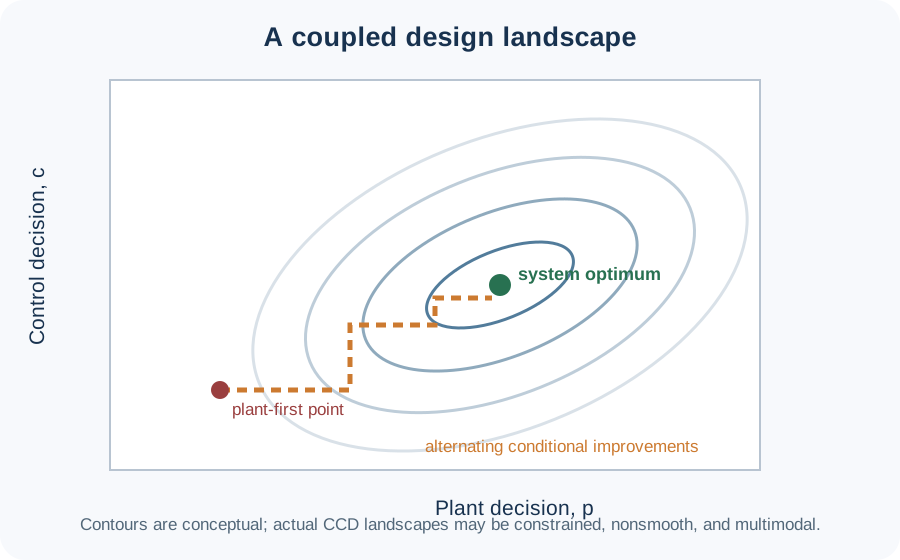
A small numerical landscape ¶ The following teaching model represents a plant choice p p p c c c
J ( p , c ) = ( p − 1.8 ) 2 + 1.4 [ c − ( 1.2 − 0.65 p ) ] 2 + 0.15 p c . J(p,c)=\left(p-1.8\right)^2+1.4\left[c-(1.2-0.65p)\right]^2+0.15pc. J ( p , c ) = ( p − 1.8 ) 2 + 1.4 [ c − ( 1.2 − 0.65 p ) ] 2 + 0.15 p c . It is not a suspension model; it is a visualization of coupled preferences. The controller preferred at one p p p
import numpy as np

def system_objective(p, c):
    return (p - 1.8)**2 + 1.4*(c - (1.2 - 0.65*p))**2 + 0.15*p*c

p_grid = np.linspace(0.0, 3.0, 301)
c_grid = np.linspace(-1.0, 2.0, 301)
P, C = np.meshgrid(p_grid, c_grid)
J = system_objective(P, C)
i = np.unravel_index(np.argmin(J), J.shape)
print(f"Grid-search CCD optimum: p={P[i]:.3f}, c={C[i]:.3f}, J={J[i]:.3f}")
p = linspace(0,3,301);
c = linspace(-1,2,301);
[P,C] = meshgrid(p,c);
J = (P-1.8).^2 + 1.4.*(C-(1.2-0.65.*P)).^2 + 0.15.*P.*C;
[Jmin,idx] = min(J(:));
fprintf('CCD optimum: p = %.3f, c = %.3f, J = %.3f\n', ...
P(idx), C(idx), Jmin);Never claim a CCD benefit by comparing an optimized integrated design with a poorly tuned sequential baseline. Retune the controller for every plant baseline, use equivalent models and constraints, and report solver tolerances and initialization.
Activity 1.5: construct a fair baseline ¶ Use the coupled objective introduced above,
J ( p , c ) = ( p − 1.8 ) 2 + 1.4 [ c − ( 1.2 − 0.65 p ) ] 2 + 0.15 p c , J(p,c)=(p-1.8)^2+1.4\left[c-(1.2-0.65p)\right]^2+0.15pc, J ( p , c ) = ( p − 1.8 ) 2 + 1.4 [ c − ( 1.2 − 0.65 p ) ] 2 + 0.15 p c , with identical bounds and feasibility constraints for every comparison:
0 ≤ p ≤ 3 , − 1 ≤ c ≤ 2 , p + 0.5 c ≤ 2.2. 0\leq p\leq 3, \qquad -1\leq c\leq 2, \qquad p+0.5c\leq 2.2. 0 ≤ p ≤ 3 , − 1 ≤ c ≤ 2 , p + 0.5 c ≤ 2.2. The plant team first minimizes the plant-only metric
J p ( p ) = ( p − 1 ) 2 + 0.10 p 2 J_p(p)=(p-1)^2+0.10p^2 J p ( p ) = ( p − 1 ) 2 + 0.10 p 2 to obtain the frozen sequential plant p s e q p_{\mathrm{seq}} p seq
Untuned baseline: ( p s e q , c 0 ) (p_{\mathrm{seq}},c_0) ( p seq , c 0 ) c 0 = 0 c_0=0 c 0 = 0
Fair sequential baseline: freeze p s e q p_{\mathrm{seq}} p seq c s e q = arg min c J ( p s e q , c ) c_{\mathrm{seq}}=\arg\min_c J(p_{\mathrm{seq}},c) c seq = arg min c J ( p seq , c )
CCD design: solve ( p c c d , c c c d ) = arg min p , c J ( p , c ) (p_{\mathrm{ccd}},c_{\mathrm{ccd}})=\arg\min_{p,c}J(p,c) ( p ccd , c ccd ) = arg min p , c J ( p , c )
Compute p s e q p_{\mathrm{seq}} p seq 10-3 in both variables.
Separate the apparent improvement into a controller-tuning gap , J ( p s e q , c 0 ) − J ( p s e q , c s e q ) J(p_{\mathrm{seq}},c_0)-J(p_{\mathrm{seq}},c_{\mathrm{seq}}) J ( p seq , c 0 ) − J ( p seq , c seq ) true CCD gap , J ( p s e q , c s e q ) − J ( p c c d , c c c d ) J(p_{\mathrm{seq}},c_{\mathrm{seq}})-J(p_{\mathrm{ccd}},c_{\mathrm{ccd}}) J ( p seq , c seq ) − J ( p ccd , c ccd )
Quantify the baseline bias using
overstatement = 100 [ J ( p s e q , c 0 ) − J c c d J ( p s e q , c s e q ) − J c c d − 1 ] % . \text{overstatement}=100\left[\frac{J(p_{\mathrm{seq}},c_0)-J_{\mathrm{ccd}}}{J(p_{\mathrm{seq}},c_{\mathrm{seq}})-J_{\mathrm{ccd}}}-1\right]\%. overstatement = 100 [ J ( p seq , c seq ) − J ccd J ( p seq , c 0 ) − J ccd − 1 ] %. Validate all three designs without retuning using the same perturbed score
J v a l ( p , c ) = J ( p , c ) + 0.10 p 2 + 0.20 c 2 . J_{\mathrm{val}}(p,c)=J(p,c)+0.10p^2+0.20c^2. J val ( p , c ) = J ( p , c ) + 0.10 p 2 + 0.20 c 2 . Report ( p , c ) (p,c) ( p , c ) 2.2 − p − 0.5 c 2.2-p-0.5c 2.2 − p − 0.5 c J J J J v a l J_{\mathrm{val}} J val