1.3 Plant-Control Design Coupling
What coupling means ¶ Plant-control coupling exists when a decision on one side changes the value, feasibility, or preferred setting of decisions on the other side. Coupling may enter through dynamics, constraints, objectives, information, or architecture.
For the quarter car, let p = [ k s , c s , F max ] T p=[k_s,c_s,F_{\max}]^T p = [ k s , c s , F m a x ] T c c c
J ( p , c ) = w a ∫ 0 T z ¨ s ( t ) 2 d t + w u ∫ 0 T u ( t ) 2 d t + w m m a ( F max ) , J(p,c)=w_a\int_0^T \ddot z_s(t)^2\,dt
+w_u\int_0^T u(t)^2\,dt+w_m m_a(F_{\max}), J ( p , c ) = w a ∫ 0 T z ¨ s ( t ) 2 d t + w u ∫ 0 T u ( t ) 2 d t + w m m a ( F m a x ) , subject to
∣ z s − z u ∣ ≤ z max , ∣ u ∣ ≤ F max , |z_s-z_u|\leq z_{\max},\qquad |u|\leq F_{\max}, ∣ z s − z u ∣ ≤ z m a x , ∣ u ∣ ≤ F m a x , and the closed-loop equations. The actuator rating is simultaneously a plant variable, a control bound, a mass/cost contributor, and a feasibility mechanism. That is strong coupling.
Five coupling channels ¶ Dynamic coupling: plant variables change poles, zeros, modes, and nonlinear behavior.
Authority coupling: actuator size and placement change reachable forces or moments.
Information coupling: sensor choices change observability, noise, and delay.
Constraint coupling: control action activates physical limits such as stress, temperature, travel, or power.
Economic coupling: control hardware and operating effort affect capital and lifecycle cost.
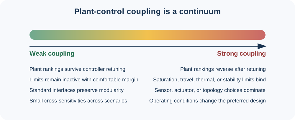
Weak and strong coupling ¶ Coupling is not binary. A practical diagnostic asks whether the controller-optimal design map
c ∗ ( p ) = arg min c J ( p , c ) c^*(p)=\arg\min_c J(p,c) c ∗ ( p ) = arg c min J ( p , c ) changes substantially over the physical design space, and whether the reduced objective
J ^ ( p ) = J ( p , c ∗ ( p ) ) \widehat J(p)=J\left(p,c^*(p)\right) J ( p ) = J ( p , c ∗ ( p ) ) has a different minimizer than a plant-only objective. Large cross-sensitivities
∂ 2 J ∂ p ∂ c \frac{\partial^2 J}{\partial p\,\partial c} ∂ p ∂ c ∂ 2 J are one clue, but active constraints and discrete architecture changes can create important coupling even when local derivatives look small.
Strong coupling often appears near a bottleneck: actuator saturation, a flexible mode, a travel limit, a thermal ceiling, a sensor blind spot, or a stability boundary. If feedback never approaches a plant-dependent limit, integrated optimization may offer little improvement.
Coupling is operating-condition dependent ¶ A plant and controller may be weakly coupled in routine operation but strongly coupled during gusts, maneuvers, faults, or extreme sea states. A suspension sized on smooth roads may appear insensitive to actuator authority; the same design may saturate over a sharp road event. CCD studies must therefore include the operating conditions that drive design decisions.
A first coupling test ¶ Before launching a large optimization:
choose several plausible plant designs;
retune the controller for each design;
record system performance and active constraints;
compare rankings before and after retuning; and
perturb actuator and information assumptions.
If plant rankings reverse, active constraints migrate, or the controller changes sharply, the problem is a strong CCD candidate.
Activity 1.3: identify the coupling channel ¶ A single-link robot must carry a 5 kg payload while tracking with closed-loop bandwidth ω b = 10 \omega_b=10 ω b = 10 L ∈ { 0.60 , 0.90 } L\in\{0.60,0.90\} L ∈ { 0.60 , 0.90 } N ∈ { 30 , 50 } N\in\{30,50\} N ∈ { 30 , 50 } μ = 3 \mu=3 μ = 3 τ m , max = 2.5 \tau_{m,\max}=2.5 τ m , m a x = 2.5 α = 2 \alpha=2 α = 2 2 ^2 2
For each architecture, calculate
m ℓ = μ L , J = 1 3 m ℓ L 2 + m p L 2 , m_\ell=\mu L, \qquad J=\frac{1}{3}m_\ell L^2+m_pL^2, m ℓ = μL , J = 3 1 m ℓ L 2 + m p L 2 , τ r e q = m ℓ g L 2 + m p g L + J α , ω 1 = 50 ( 0.60 L ) 2 , \tau_{\mathrm{req}}=m_\ell g\frac{L}{2}+m_pgL+J\alpha, \qquad \omega_1=50\left(\frac{0.60}{L}\right)^2, τ req = m ℓ g 2 L + m p gL + J α , ω 1 = 50 ( L 0.60 ) 2 , M τ = N τ m , max τ r e q , P c u = 8 ( 0.35 τ r e q N ) 2 , M_\tau=\frac{N\tau_{m,\max}}{\tau_{\mathrm{req}}}, \qquad P_{\mathrm{cu}}=8\left(\frac{0.35\tau_{\mathrm{req}}}{N}\right)^2, M τ = τ req N τ m , m a x , P cu = 8 ( N 0.35 τ req ) 2 , and the delay-induced phase lag
ϕ d = ω b τ s 180 π . \phi_d=\omega_b\tau_s\frac{180}{\pi}. ϕ d = ω b τ s π 180 . Use the following requirements and costs:
Requirement or component Value Flexible-mode separation ω 1 / ω b ≥ 3 \omega_1/\omega_b\geq 3 ω 1 / ω b ≥ 3 Actuator authority M τ ≥ 1.25 M_\tau\geq 1.25 M τ ≥ 1.25 Motor thermal limit P c u ≤ 1.2 P_{\mathrm{cu}}\leq 1.2 P cu ≤ 1.2 Delay limit ϕ d ≤ 1 5 ∘ \phi_d\leq 15^\circ ϕ d ≤ 1 5 ∘ Fast sensor τ s = 5 \tau_s=5 τ s = 5 Slow sensor τ s = 30 \tau_s=30 τ s = 30 Architecture cost C = 500 + 12 N + C s C=500+12N+C_s C = 500 + 12 N + C s
Evaluate all eight combinations of ( L , N , τ s ) (L,N,\tau_s) ( L , N , τ s ) ω 1 / ω b \omega_1/\omega_b ω 1 / ω b M τ M_\tau M τ P c u P_{\mathrm{cu}} P cu ϕ d \phi_d ϕ d
For every failed constraint, identify the primary coupling channel: dynamic , authority , information , constraint , or economic . Explain why motor heating is both authority-related and constraint-related.
Find the least-cost feasible architecture. Then repeat only the affected calculations for ω b = 7 \omega_b=7 ω b = 7
State which physical or information decision most strongly controls the feasible set. Support the claim with one numerical margin, not only a verbal argument.
Use g = 9.81 g=9.81 g = 9.81 2 ^2 2