0.4 Optimization and Discretization

Optimization provides a precise language for stating what may change, what should improve, and what conditions must remain satisfied. Discretization then converts continuous-time functions into finite vectors that numerical algorithms can manipulate.

Basic optimization language¶

Optimization problem structure¶

A constrained optimization problem can be written as

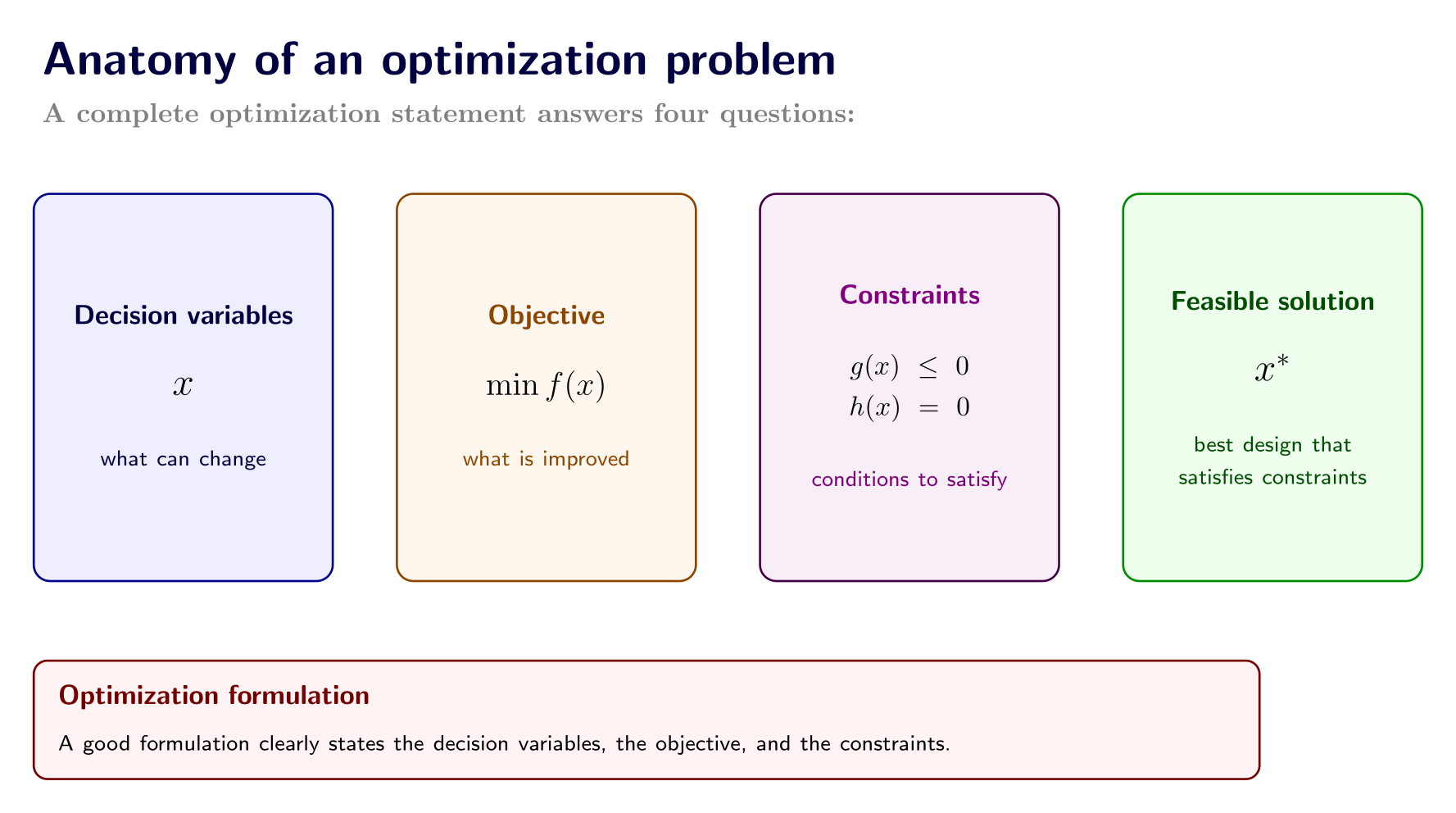
\begin{aligned} \min_{\mathbf{x}}\quad & f(\mathbf{x})\\ \text{subject to}\quad & g_i(\mathbf{x})\leq 0, && i=1,\ldots,n_g,\\ & h_j(\mathbf{x})=0, && j=1,\ldots,n_h,\\ & \mathbf{x}^{L}\leq\mathbf{x}\leq\mathbf{x}^{U}. \end{aligned}

Decision variables enter an objective and constraints to produce a feasible optimization solution. — The principal parts of an optimization problem.

Core terms¶

Decision variables: Quantities the optimizer is allowed to change.
Objective function: The quantity being minimized or maximized.
Constraints: Conditions that a solution must satisfy.
Feasible point: A point that satisfies every constraint.
Feasible region: The set of all feasible points.
Optimal point: A feasible point with the best objective value, according to the stated problem.

Example optimization statement¶

A simple engineering design problem is

\begin{aligned} \min_{m,k}\quad & J(m,k)=m^2+0.5k^2\\ \text{subject to}\quad & m\geq0.1,\\ &10\leq k\leq1000. \end{aligned}

This statement specifies the quantities being chosen, the performance measure being improved, and the bounds that must hold.

How CCD builds on this structure¶

A CCD problem uses the same optimization language but adds dynamic-system structure. Its decision variables include plant and controller quantities, while its constraints often include state equations over time:

\dot{\mathbf{x}}=\mathbf{f}(\mathbf{x},\mathbf{u},\mathbf{x}_p,\mathbf{x}_c,t).

The objective may also depend on an entire trajectory rather than on a few static variables.

Discretization and sampled variables¶

Why discretization is needed¶

Many CCD problems are naturally continuous in time. Numerical optimizers, however, operate on finite-dimensional vectors rather than on arbitrary continuous functions. Continuous trajectories must therefore be approximated by samples or coefficients.

Time mesh¶

Divide a time interval into nodes:

t_0<t_1<\cdots<t_N.

The width of interval $i$ is

\Delta t_i=t_{i+1}-t_i.

The mesh is uniform if every $\Delta t_i$ is equal and nonuniform otherwise.

Sampled states and controls¶

At each node, approximate the state and control by

\mathbf{x}_i\approx\mathbf{x}(t_i), \qquad \mathbf{u}_i\approx\mathbf{u}(t_i).

If the control is scalar, its sampled trajectory becomes the finite vector

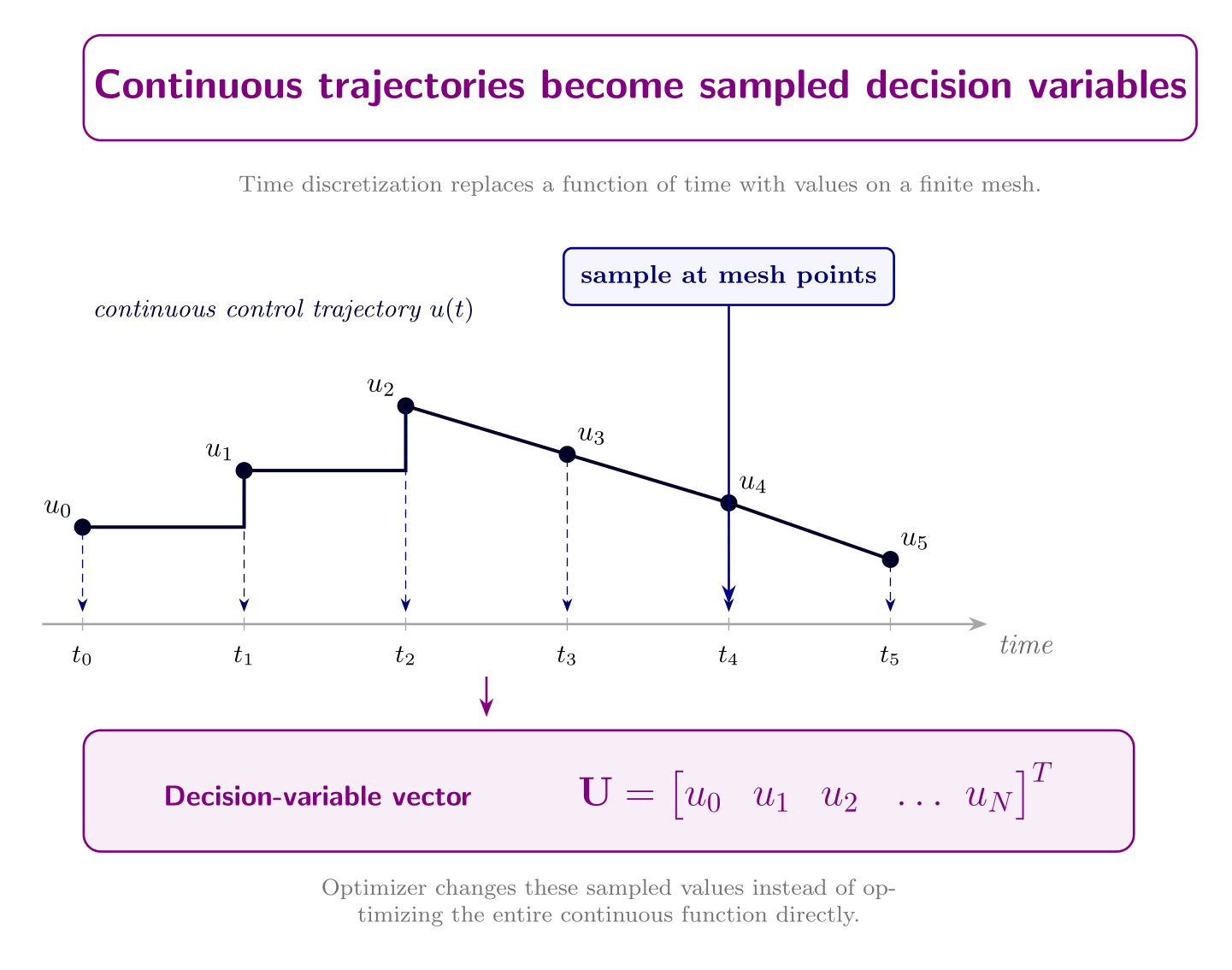
\mathbf{U}= \begin{bmatrix} u_0&u_1&\cdots&u_N \end{bmatrix}^{T}.

Values of a continuous control trajectory sampled at time nodes form a finite decision vector. — A continuous trajectory becomes a finite vector when sampled on a time mesh.

From differential equations to algebraic constraints¶

Discretization must also enforce the system dynamics. A simple forward-Euler approximation is

\dot{\mathbf{x}}(t_i) \approx \frac{\mathbf{x}_{i+1}-\mathbf{x}_i}{\Delta t_i}.

Substituting this approximation into

\dot{\mathbf{x}}=\mathbf{f}(\mathbf{x},\mathbf{u},t)

gives the algebraic relation

\mathbf{x}_{i+1}-\mathbf{x}_i -\Delta t_i\mathbf{f}(\mathbf{x}_i,\mathbf{u}_i,t_i)=\mathbf{0}.

Higher-accuracy methods use different approximations, but the central idea remains: a continuous-time model becomes a finite set of algebraic equations.

Why this matters later¶

This conversion underlies direct shooting, multiple shooting, direct transcription, and collocation. It also introduces important numerical questions:

Is the mesh fine enough to represent the trajectory accurately?
Does the discrete objective approximate the intended continuous objective?
Do the discrete dynamics enforce the original ODE closely enough?
Does refining the mesh change the apparent optimum?

Activity 0.5: Discretized Minimum-Energy Control Solved by Linear Algebra¶

Activity 0.5: Discretized Minimum-Energy Control Solved by Linear Algebra

Consider the double-integrator system

\dot{x}_1=x_2, \qquad \dot{x}_2=u, \qquad x_1(0)=x_2(0)=0.

Use a time horizon $T=1$ divided into four equal intervals of length $h=1/4$ . Assume the control is piecewise constant:

u(t)=u_i, \qquad t\in[ih,(i+1)h), \qquad i=0,1,2,3.

Use the exact zero-order-hold discrete dynamics

\begin{bmatrix}x_{1,i+1}\\x_{2,i+1}\end{bmatrix} = \begin{bmatrix}1&h\\0&1\end{bmatrix} \begin{bmatrix}x_{1,i}\\x_{2,i}\end{bmatrix} + \begin{bmatrix}h^2/2\\h\end{bmatrix}u_i.

The terminal requirements are

x_1(1)=1, \qquad x_2(1)=0,

and the discrete control-effort objective is

J=h\sum_{i=0}^{3}u_i^2.

Propagate the dynamics symbolically and express the terminal state as
$\mathbf{x}_4=G\mathbf{U}, \qquad \mathbf{U}=\begin{bmatrix}u_0&u_1&u_2&u_3\end{bmatrix}^{T}.$
Write the terminal requirements as $G\mathbf{U}=\mathbf{b}$ .
Show that the problem is a minimum-norm equality-constrained quadratic problem.
Using Lagrange multipliers, prove that
$\mathbf{U}^*=G^T(GG^T)^{-1}\mathbf{b}.$
Compute all four optimal control values.
Compute the complete state trajectory at the five time nodes.
Verify the terminal conditions exactly.
Repeat the derivation for an arbitrary number $N$ of equal intervals.
Explain how the dimensions of $G$ , $\mathbf{U}$ , and $\mathbf{b}$ change with $N$ .
Compare the discrete solution with the continuous minimum-energy control obtained by calculus of variations or an optimal-control solver.