0.2 Calculus and Linear Algebra

Calculus describes rates, sensitivities, and accumulated quantities. Linear algebra provides the language for systems with many states, inputs, outputs, and design variables. Together, they support nearly every CCD formulation and numerical method in this course.

Derivatives and partial derivatives¶

Single-variable derivatives¶

The derivative of a scalar function $f(x)$ is written

\frac{df}{dx}.

It measures the rate at which $f$ changes when $x$ changes. In optimization, a derivative indicates how an objective or constraint responds to a small adjustment in a decision variable.

f(x)=x^2,

then

\frac{df}{dx}=2x.

The second derivative,

\frac{d^2f}{dx^2},

measures how the slope changes and provides information about curvature.

Partial derivatives¶

When a function depends on several variables, a partial derivative describes its sensitivity to one variable while the others are held fixed:

\frac{\partial f}{\partial x_i}.

For

J(k,c)=k^2+2c^2-kc,

the partial derivatives are

\frac{\partial J}{\partial k}=2k-c, \qquad \frac{\partial J}{\partial c}=4c-k.

Gradient¶

The gradient collects the first partial derivatives of a scalar function into a vector:

\nabla J(\mathbf{x})= \begin{bmatrix} \dfrac{\partial J}{\partial x_1}\\ \dfrac{\partial J}{\partial x_2}\\ \vdots\\ \dfrac{\partial J}{\partial x_n} \end{bmatrix}.

For the function $J(k,c)$ ,

\nabla J(k,c)= \begin{bmatrix} 2k-c\\ 4c-k \end{bmatrix}.

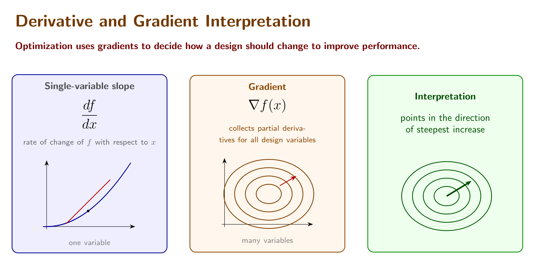
A derivative gives a single-variable slope, while a gradient collects partial derivatives and points toward steepest increase. — Derivatives and gradients provide the change information used by many optimization algorithms.

Chain rule¶

If one variable depends on another,

z=f(y),\qquad y=g(x),

the chain rule propagates derivatives through the nested relationship:

\frac{dz}{dx}=\frac{dz}{dy}\frac{dy}{dx}.

This idea is fundamental to sensitivity analysis and automatic differentiation.

Jacobian and Hessian¶

For a vector-valued function

\mathbf{r}(\mathbf{x})= \begin{bmatrix} r_1(\mathbf{x})\\ r_2(\mathbf{x})\\ \vdots\\ r_m(\mathbf{x}) \end{bmatrix},

the Jacobian is the matrix of first derivatives:

\frac{\partial\mathbf{r}}{\partial\mathbf{x}}= \begin{bmatrix} \dfrac{\partial r_1}{\partial x_1} & \cdots & \dfrac{\partial r_1}{\partial x_n}\\ \vdots & \ddots & \vdots\\ \dfrac{\partial r_m}{\partial x_1} & \cdots & \dfrac{\partial r_m}{\partial x_n} \end{bmatrix}.

The Hessian of a scalar function is the matrix of its second partial derivatives. Jacobians describe the local sensitivity of vector equations; Hessians describe the local curvature of scalar objectives or constraints.

Example: gradient of a design objective¶

Let

J(m,k)=m^2+0.5k^2-mk.

Then

\frac{\partial J}{\partial m}=2m-k, \qquad \frac{\partial J}{\partial k}=k-m,

\nabla J(m,k)= \begin{bmatrix} 2m-k\\ k-m \end{bmatrix}.

This calculation is the basic language of gradient-based optimization.

Integration and numerical integration¶

Definite integrals as accumulated quantities¶

A definite integral accumulates a quantity over an interval:

\int_{t_0}^{t_f}q(t)\,dt.

In engineering, integrals can represent accumulated energy, work, fuel, tracking error, or control effort. For example,

J=\int_0^T u(t)^2\,dt

is a common measure of control effort.

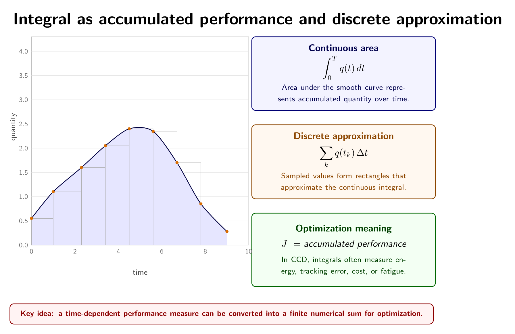
A continuous curve and sampled values illustrate an integral and its numerical approximation. — A definite integral measures accumulated area; numerical methods approximate it using sampled values.

Numerical integration¶

When time is discretized at $t_0,t_1,\ldots,t_N$ , a left-rectangle approximation is

\int_{t_0}^{t_f}q(t)\,dt \approx \sum_{i=0}^{N-1}q_i\Delta t_i,

where $q_i\approx q(t_i)$ and $\Delta t_i=t_{i+1}-t_i$ .

The trapezoidal rule uses both endpoints of each interval:

\int_{t_0}^{t_f}q(t)\,dt \approx \sum_{i=0}^{N-1}\frac{\Delta t_i}{2}(q_i+q_{i+1}).

For the control-effort objective,

J=\int_0^T u(t)^2\,dt,

the trapezoidal approximation is

J\approx \sum_{i=0}^{N-1}\frac{\Delta t_i}{2} \left(u_i^2+u_{i+1}^2\right).

This form appears later in direct-transcription methods.

Linear algebra¶

Vectors, matrices, and dimensions¶

A vector is an ordered list of numbers; a matrix is a rectangular array:

\mathbf{x}= \begin{bmatrix} x_1\\x_2\\x_3 \end{bmatrix}, \qquad A= \begin{bmatrix} 1&0\\2&3 \end{bmatrix}.

If $A\in\mathbb{R}^{m\times n}$ , then $A$ has $m$ rows and $n$ columns. The product $A\mathbf{x}$ is defined only when the number of columns in $A$ equals the number of components in $\mathbf{x}$ .

Important operations include vector and matrix addition, scalar multiplication, matrix multiplication, transpose $A^T$ , and—when it exists—the inverse $A^{-1}$ .

Identity matrices and linear systems¶

The identity matrix satisfies

I\mathbf{x}=\mathbf{x}.

A linear system has the form

A\mathbf{x}=\mathbf{b}.

If $A$ is square and nonsingular, the mathematical solution can be written $\mathbf{x}=A^{-1}\mathbf{b}$ . In computation, however, one normally uses a linear-system solver rather than forming the inverse explicitly.

Norms¶

A norm measures vector size. The Euclidean norm is

\|\mathbf{x}\|_2=\sqrt{x_1^2+x_2^2+\cdots+x_n^2}.

Norms appear in convergence tests, regularization terms, error measures, and engineering-performance metrics.

Eigenvalues and eigenvectors¶

An eigenvalue–eigenvector pair satisfies

A\mathbf{v}=\lambda\mathbf{v}.

In state-space models, eigenvalues help characterize dynamic behavior and stability.

Positive definiteness¶

A symmetric matrix $Q$ is positive definite if

\mathbf{z}^{T}Q\mathbf{z}>0 \qquad\text{for every nonzero }\mathbf{z}.

Positive-definite matrices occur frequently in quadratic objectives and Lyapunov analysis.

Activity 0.1: Composite Engineering Functions, Gradients, and Hessians¶

Activity 0.1: Composite Engineering Functions, Gradients, and Hessians

For a mass-spring-damper system, define

\omega_n(m,k)=\sqrt{\frac{k}{m}}, \qquad \zeta(m,k,c)=\frac{c}{2\sqrt{km}}.

Consider the dimensionless design objective

J(m,k,c)= \left(\frac{\omega_n-\omega_d}{\omega_d}\right)^2 +\beta\left(\frac{\zeta-\zeta_d}{\zeta_d}\right)^2 +\gamma\left(\frac{m}{m_{\mathrm{ref}}}\right)^2,

where

\omega_d=4\ \mathrm{rad/s}, \qquad \zeta_d=0.7, \qquad \beta=2, \qquad \gamma=0.05, \qquad m_{\mathrm{ref}}=2\ \mathrm{kg}.

Derive
$\frac{\partial\omega_n}{\partial m}, \qquad \frac{\partial\omega_n}{\partial k}.$
Derive
$\frac{\partial\zeta}{\partial m}, \qquad \frac{\partial\zeta}{\partial k}, \qquad \frac{\partial\zeta}{\partial c}.$
Use the chain rule to derive the complete gradient $\nabla J(m,k,c)$ .
Evaluate $J$ and $\nabla J$ at
$m=2\ \mathrm{kg}, \qquad k=24\ \mathrm{N/m}, \qquad c=5\ \mathrm{N\,s/m}.$
Let
$\mathbf{d}=\frac{1}{\sqrt{6}} \begin{bmatrix}1\\-2\\1\end{bmatrix}.$
Compute the directional derivative
$D_{\mathbf{d}}J=\nabla J^T\mathbf{d}.$
Derive the $3\times3$ Hessian matrix $H_J(m,k,c)$ .
Evaluate the eigenvalues of the Hessian at the stated design and determine whether $J$ is locally convex there.
Verify the analytical gradient using central finite differences with step sizes
$h\in\{10^{-2}, 10^{-4}, 10^{-6}, 10^{-8}\}.$

Activity 0.2: Numerical Integration and Observed Convergence Order¶

Activity 0.2: Numerical Integration and Observed Convergence Order

Consider

q(t)=e^{-t}\sin(3t), \qquad 0\leq t\leq2,

and define

I=\int_0^2 q(t)^2\,dt.

Evaluate $I$ analytically.
Approximate $I$ using:
1. the left-rectangle rule;
2. the midpoint rule;
3. the composite trapezoidal rule; and
4. composite Simpson’s rule.
Use
$N\in\{10, 20, 40, 80, 160\}$
equal subintervals.
For each method, compute the absolute error
$e_N=|I_N-I|.$
Estimate the observed convergence order using
$p_N=\frac{\log(e_N/e_{2N})}{\log 2}.$
Compare the observed orders with the theoretical orders of the four methods.
Derive the composite trapezoidal approximation in matrix form:
$I_N=\mathbf{w}^T\mathbf{q}^{\,2},$
where $\mathbf{w}$ is the quadrature-weight vector.
Explain why a highly accurate state trajectory does not automatically guarantee a highly accurate integral performance measure if the quadrature rule is inconsistent with the trajectory approximation.

Activity 0.3: Linear Algebra, Modal Coordinates, and Positive Definiteness

Consider the undamped two-degree-of-freedom mechanical system

M\ddot{\mathbf{q}}+K\mathbf{q}=\mathbf{0},

where

M=\begin{bmatrix}2&0\\0&1\end{bmatrix}, \qquad K=\begin{bmatrix}6&-2\\-2&4\end{bmatrix}.

Verify that $M$ and $K$ are symmetric positive definite.
Solve the generalized eigenvalue problem
$K\boldsymbol{\phi}=\omega^2M\boldsymbol{\phi}.$
Compute the two natural frequencies.
Normalize the mode shapes so that
$\Phi^TM\Phi=I.$
Verify that
$\Phi^TK\Phi=\operatorname{diag}(\omega_1^2,\omega_2^2).$
Introduce modal coordinates $\mathbf{q}=\Phi\boldsymbol{\eta}$ and derive the decoupled equations of motion.
For
$\mathbf{q}(0)=\begin{bmatrix}1\\0\end{bmatrix}, \qquad \dot{\mathbf{q}}(0)=\begin{bmatrix}0\\0\end{bmatrix},$
compute the initial modal coordinates.
Derive the exact displacement response $\mathbf{q}(t)$ .
Compute the total mechanical energy
$E(t)=\frac{1}{2}\dot{\mathbf{q}}^TM\dot{\mathbf{q}} +\frac{1}{2}\mathbf{q}^TK\mathbf{q}$
and prove that it is constant.
Explain why positive definiteness of $M$ and $K$ matters physically and mathematically.

0.2 Calculus and Linear Algebra

Derivatives and partial derivatives¶

Single-variable derivatives¶

Partial derivatives¶

Gradient¶

Chain rule¶

Jacobian and Hessian¶

Example: gradient of a design objective¶

Integration and numerical integration¶

Definite integrals as accumulated quantities¶

Numerical integration¶

Linear algebra¶

Vectors, matrices, and dimensions¶

Identity matrices and linear systems¶

Norms¶

Eigenvalues and eigenvectors¶

Positive definiteness¶

Activity 0.1: Composite Engineering Functions, Gradients, and Hessians¶

Activity 0.2: Numerical Integration and Observed Convergence Order¶

Activity 0.3: Linear Algebra, Modal Coordinates, and Positive Definiteness¶