0.3 Differential Equations and State-Space Models

Dynamic systems are modeled with differential equations because their rates of change depend on current states, inputs, time, and physical parameters. CCD uses these equations both to predict system behavior and to constrain the optimization problem.

Ordinary differential equations¶

What is a differential equation?¶

A differential equation relates a function to one or more of its derivatives. A first-order ordinary differential equation (ODE) can be written

\dot{x}=f(x,u,t),

while a second-order ODE can be written

\ddot{x}=g(x,\dot{x},u,t).

The derivative order refers to the highest derivative appearing in the equation.

Mass–spring–damper example¶

A standard engineering model is

m\ddot{x}+c\dot{x}+kx=u(t),

where

$m$ is mass,
$c$ is the damping coefficient,
$k$ is spring stiffness, and
$u(t)$ is an external force or control input.

In a CCD problem, $m$ , $c$ , and $k$ could be plant design variables, while $u(t)$ or the parameters of a feedback law could be control design variables.

Initial conditions¶

The differential equation alone does not determine a unique trajectory. A second-order initial-value problem normally also requires displacement and velocity at the initial time:

x(0)=x_0, \qquad \dot{x}(0)=v_0.

Converting a higher-order ODE to first-order form¶

First-order state-space form is central to simulation, control, and optimal control. Define

x_1=x, \qquad x_2=\dot{x}.

The first state equation is

\dot{x}_1=x_2.

Solving the original mass–spring–damper equation for acceleration gives

\ddot{x}=-\frac{k}{m}x-\frac{c}{m}\dot{x}+\frac{1}{m}u,

so the second state equation is

\dot{x}_2=-\frac{k}{m}x_1-\frac{c}{m}x_2+\frac{1}{m}u.

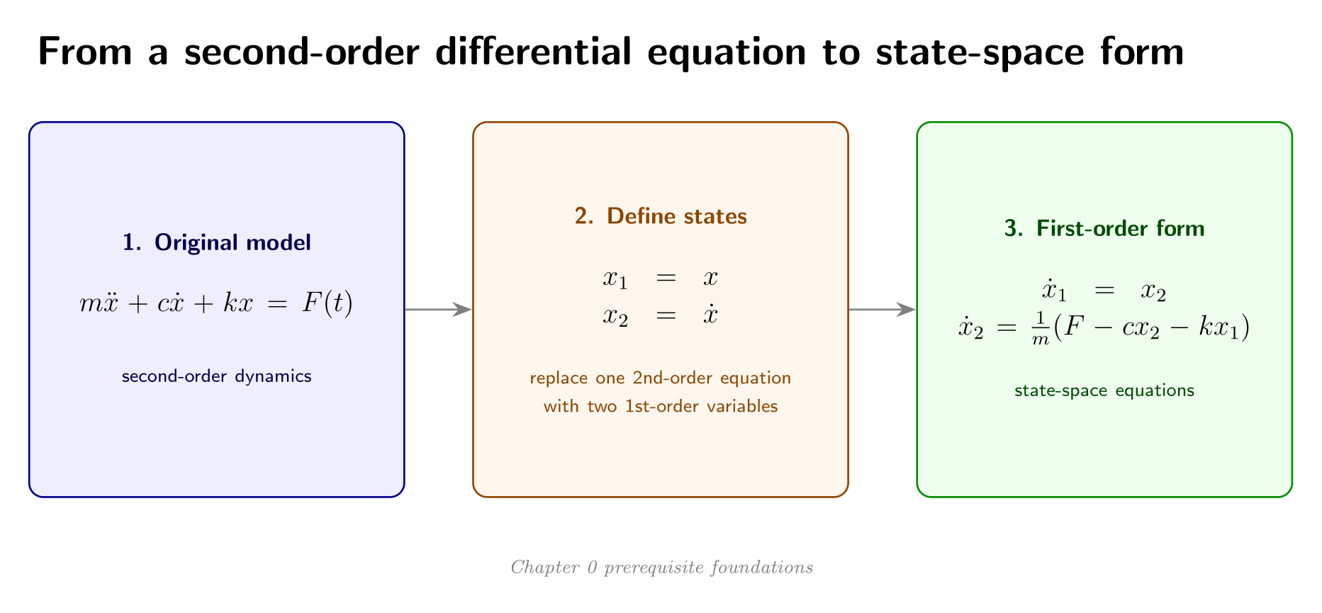
A mass-spring-damper equation is converted into two coupled first-order state equations. — Second-order engineering models are commonly rewritten as systems of first-order state equations.

Example: state conversion¶

Collect the two states in a vector:

\mathbf{x}= \begin{bmatrix} x_1\\x_2 \end{bmatrix} = \begin{bmatrix} x\\\dot{x} \end{bmatrix}.

The dynamics can then be written compactly as

\dot{\mathbf{x}}= \begin{bmatrix} x_2\\ -\dfrac{k}{m}x_1-\dfrac{c}{m}x_2+\dfrac{1}{m}u \end{bmatrix}.

This representation reappears in Chapter 2 and in later optimal-control formulations.

Introductory state-space notation¶

Nonlinear state-space form¶

A general nonlinear dynamic system is often written

\dot{\mathbf{x}}=\mathbf{f}(\mathbf{x},\mathbf{u},t), \qquad \mathbf{y}=\mathbf{h}(\mathbf{x},\mathbf{u},t),

where

$\mathbf{x}$ is the state vector,
$\mathbf{u}$ is the input vector,
$\mathbf{y}$ is the output vector,
$\mathbf{f}$ defines the state dynamics, and
$\mathbf{h}$ maps states and inputs to outputs.

Linear state-space form¶

For a linear time-invariant system,

\dot{\mathbf{x}}=A\mathbf{x}+B\mathbf{u}, \qquad \mathbf{y}=C\mathbf{x}+D\mathbf{u}.

The matrices have compatible dimensions:

Matrix	Role
$A$	State or system matrix
$B$	Input matrix
$C$	Output matrix
$D$	Direct-feedthrough matrix

State-space notation is compact, supports multiple states and inputs, and works naturally with vector and matrix operations. It is therefore widely used in control theory and CCD.

Activity 0.4: Exact State-Space Response of a Forced Dynamic System¶

Activity 0.4: Exact State-Space Response of a Forced Dynamic System

Consider

m\ddot{x}+c\dot{x}+kx=u_0,

where $u_0$ is a constant input. Use

\begin{aligned} m&=1.5\ \mathrm{kg}, & c&=1.8\ \mathrm{N\,s/m}, & k&=12\ \mathrm{N/m},\\ u_0&=3\ \mathrm{N}, & x(0)&=0.2\ \mathrm{m}, & \dot{x}(0)&=-0.1\ \mathrm{m/s}. \end{aligned}

Define
$\mathbf{x}=\begin{bmatrix}x\\\dot{x}\end{bmatrix}$
and derive
$\dot{\mathbf{x}}=A\mathbf{x}+Bu_0.$
Compute the eigenvalues of $A$ and classify the response as underdamped, critically damped, or overdamped.
Compute the equilibrium state $\mathbf{x}_{\mathrm{eq}}$ associated with the constant input.
Define
$\widetilde{\mathbf{x}}=\mathbf{x}-\mathbf{x}_{\mathrm{eq}}$
and derive the homogeneous shifted system.
Derive
$\mathbf{x}(t)=e^{At} \left(\mathbf{x}(0)-\mathbf{x}_{\mathrm{eq}}\right) +\mathbf{x}_{\mathrm{eq}}.$
Obtain explicit scalar expressions for $x(t)$ and $\dot{x}(t)$ .
Compute the first time at which the displacement reaches its steady-state value.
Compute the maximum displacement over $0\leq t\leq5$ .
Verify the analytical solution using a numerical ODE integrator.
Repeat the numerical solution using forward Euler with
$h\in\{0.2, 0.1, 0.05, 0.025\}.$
Estimate the observed global convergence order.