0.1 Mathematical Notation and Engineering Functions

Control co-design formulations can look intimidating because they express many related ideas compactly. Becoming comfortable with the notation makes the modeling and optimization concepts in later chapters much easier to follow.

Mathematical notation and engineering variables¶

Scalars, vectors, matrices, and trajectories¶

These notes use the following conventions:

Italic lowercase letters such as $m$ , $k$ , and $t$ denote scalars.
Bold lowercase letters such as $\mathbf{x}$ and $\mathbf{u}$ denote vectors.
Uppercase letters such as $A$ , $B$ , and $C$ denote matrices.
Time-varying quantities are written explicitly, such as $x(t)$ , $\mathbf{x}(t)$ , or $u(t)$ ; these functions of time are trajectories.

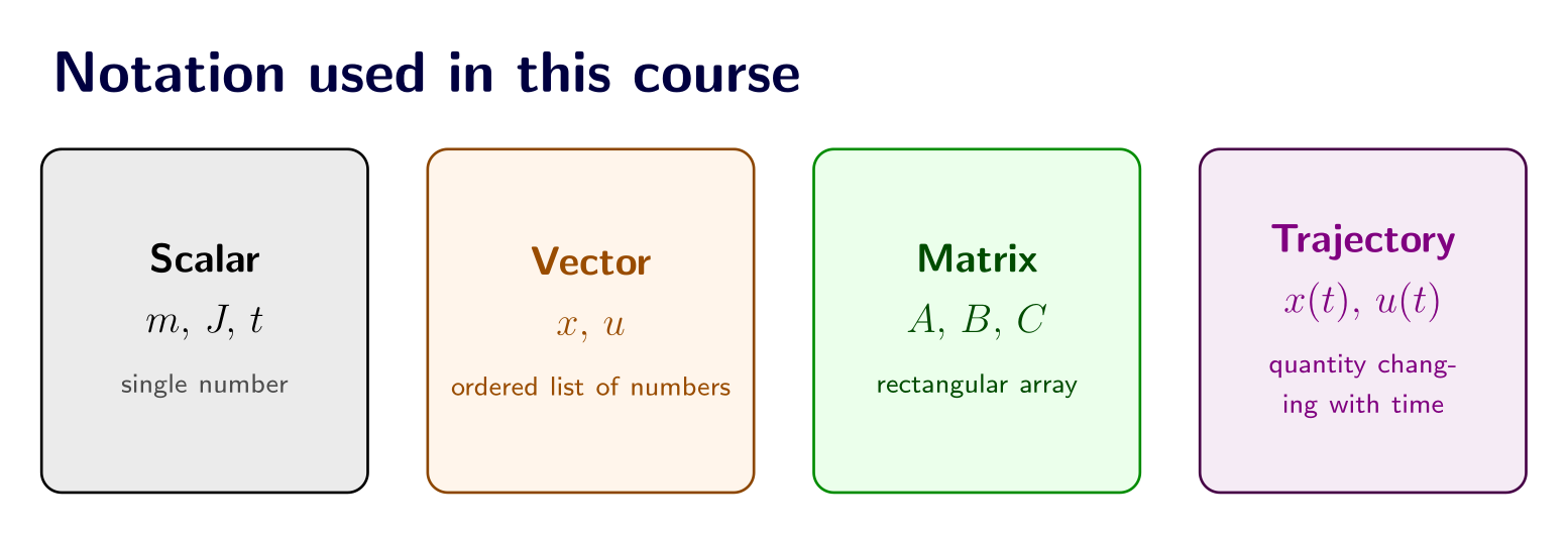
Scalars are single numbers, vectors are ordered lists, matrices are rectangular arrays, and trajectories change with time. — The main notation categories used throughout the course.

Common variables in control co-design¶

The following symbols appear frequently in later chapters:

Symbol	Meaning
$\mathbf{x}_p$	Plant design variables
$\mathbf{x}_c$	Control design variables or controller parameters
$\mathbf{x}(t)$	State trajectory
$\mathbf{u}(t)$	Control-input trajectory
$\mathbf{y}(t)$	Output trajectory or measured signals
$J$	Objective function or performance index
$g(\cdot)$	Inequality constraints
$h(\cdot)$	Equality constraints

For example, a plant-variable vector might be

\mathbf{x}_p= \begin{bmatrix} m & k & c \end{bmatrix}^{T},

while a controller-parameter vector might be

\mathbf{x}_c= \begin{bmatrix} K_p & K_i & K_d \end{bmatrix}^{T}.

Subscripts and superscripts¶

Subscripts usually identify components, samples, or categories. For example,

\mathbf{x}= \begin{bmatrix} x_1 & x_2 & \cdots & x_n \end{bmatrix}^{T}

means that $\mathbf{x}$ contains $n$ components. In a time-discretized problem, $x_i$ may instead mean the value of a variable at the $i$ th time node; the surrounding context determines the intended meaning.

Superscripts may indicate powers, algorithm iterations, or labels. The notation

\mathbf{x}^{(k)}

usually denotes the value of $\mathbf{x}$ at iteration $k$ of an algorithm, whereas $x^2$ denotes the square of a scalar.

Summation notation¶

Summation notation is common in discrete approximations and finite-dimensional optimization:

\sum_{i=1}^{N}a_i=a_1+a_2+\cdots+a_N.

If a scalar control input is sampled at $N$ points, a simple discrete measure of control effort is

J=\sum_{i=1}^{N}u_i^2.

The index $i$ can identify time nodes, operating conditions, load cases, uncertain scenarios, or experimental trials.

Sets, bounds, and intervals¶

Variable bounds are often written componentwise:

\mathbf{x}^{L}\leq\mathbf{x}\leq\mathbf{x}^{U},

where $\mathbf{x}^{L}$ and $\mathbf{x}^{U}$ are lower and upper bounds. The notation $t\in[t_0,t_f]$ means that time belongs to the closed interval from $t_0$ to $t_f$ .

Functions and engineering relationships¶

A function maps one quantity to another. In engineering, functions describe relationships among design variables, states, inputs, outputs, objectives, and constraints.

Single-variable and multivariable functions¶

A single-variable function has the form

y=f(x),

whereas a multivariable function may have the form

J=f(x_1,x_2,\ldots,x_n).

For example,

J(k,c)=k^2+2c^2-kc

depends on two design variables: stiffness $k$ and damping $c$ .

Explicit and implicit relationships¶

An explicit relationship directly gives one variable as a function of others, such as

y=3x+2.

An implicit relationship combines variables in one equation, such as

x^2+y^2=1.

Both forms occur in engineering models and constraints.

Linear, affine, and nonlinear relationships¶

A linear function preserves scaling and addition. A relationship such as $y=ax$ is linear, while

y=ax+b

is affine because of the constant offset $b$ . A relationship such as

y=x^2+\sin(x)

is nonlinear. Most CCD problems are nonlinear because plant and controller decisions interact through nonlinear dynamics, constraints, and performance measures.

Time-dependent functions¶

Dynamic systems are described using time-dependent functions such as $\mathbf{x}(t)$ and $\mathbf{u}(t)$ . A trajectory is not one number: it assigns a value at every time in an interval. Later numerical methods will replace these continuous functions with finite sets of samples or coefficients.