0.5 Computational Preparation and Readiness Project
CCD studies combine mathematical models with numerical simulation and optimization. You do not need advanced software-development experience to begin, but you should be comfortable reading and modifying short computational scripts.
Minimal MATLAB or Python preparation
Before continuing, you should be able to:
define scalars, vectors, and matrices;
write and call a simple function;
evaluate a mathematical formula;
simulate an ODE numerically;
plot a result; and
compute a discrete objective function.
A simple computational workflow
A basic modeling study follows a repeatable sequence:
Define parameters and initial conditions.
Write the model equations.
Simulate the model and plot the results.
Evaluate one or more performance measures.
Refine the model, parameters, or numerical settings.
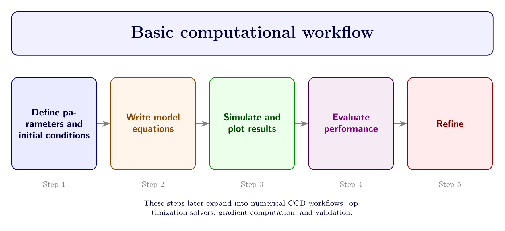
A basic workflow for modeling and simulation. Later CCD workflows add optimization solvers, gradient computation, uncertainty studies, and validation.
Python example
The following script defines a mass–spring–damper model and integrates it numerically. It is a preparation exercise rather than a full CCD implementation.
import numpy as np
from scipy.integrate import solve_ivp
import matplotlib.pyplot as plt

m = 1.0
c = 0.4
k = 4.0


def model(t, x):
    u = 1.0
    x1, x2 = x
    dx1 = x2
    dx2 = -(k / m) * x1 - (c / m) * x2 + (1 / m) * u
    return [dx1, dx2]


sol = solve_ivp(model, [0, 10], [0, 0], max_step=0.02)

plt.plot(sol.t, sol.y[0, :])
plt.xlabel("time")
plt.ylabel("displacement")
plt.show()
The script performs four basic tasks:
specifies the model parameters , , and ;
defines the first-order state equations;
integrates the equations from an initial state; and
plots the displacement trajectory.
MATLAB example
An analogous MATLAB script is
m = 1.0;
c = 0.4;
k = 4.0;

f = @(t,x) [x(2);
           -(k/m)*x(1) - (c/m)*x(2) + 1/m];

[t,x] = ode45(f,[0 10],[0;0]);

plot(t,x(:,1))
xlabel('time')
ylabel('displacement')
Both implementations express the same mathematical model. The syntax differs, but the modeling workflow is unchanged.
Computing a discrete performance measure
Suppose the continuous control-effort objective is
After sampling on a time grid, a trapezoidal approximation can be computed in Python with
J = np.trapezoid(u**2, t)or in MATLAB with
J = trapz(t, u.^2);This simple pattern—simulate a trajectory, compute a performance measure, and compare alternatives—later becomes part of a numerical optimization loop.
Readiness mini-project
Before moving to Chapter 1, model and simulate a mass–spring–damper system and identify how its quantities would appear in a CCD formulation.
Suggested tasks
Choose values for , , and .
Write the second-order ODE and convert it to first-order state-space form.
Select initial conditions and a force input .
Simulate displacement and velocity.
Plot both state trajectories.
Compute at least one performance measure, such as peak displacement, RMS displacement, or control effort.
Explain which quantities could become decision variables and which conditions could become constraints.
Connection to a CCD formulation
| CCD element | Mass–spring–damper example |
|---|---|
| Plant variables | , , and |
| Control variables | Force-input history or controller gains |
| States | Displacement and velocity |
| Possible objectives | Vibration suppression, control effort, or a weighted combination |
| Possible constraints | Actuator-force limits, displacement bounds, or parameter bounds |
Activity 0.6: State and Parameter Sensitivities for a Readiness Mini-Project
Activity 0.6: State and Parameter Sensitivities for a Readiness Mini-Project
Consider the mass-spring-damper system
with
The plant parameters and state vector are
Define the performance measure
Derive the state-space model
Define the parameter-sensitivity vectors
Derive the sensitivity equations
Derive the initial conditions for both sensitivity vectors.
Derive and in terms of the state and sensitivity trajectories.
Simulate the state and sensitivity equations simultaneously at
Verify both derivatives using central finite differences.
Investigate the finite-difference error for
Use the computed gradient to perform ten steepest-descent iterations with a backtracking line search, subject to
Report the final design, objective value, gradient norm, and state response.
Explain how this mini-project combines the main prerequisite topics of Chapter 0 and prepares students for later CCD formulations.