State Inequality Path Constraints and Direct Collocation
This section continues the treatment of path constraints by focusing on state inequality path constraints and their numerical implementation. These constraints are challenging because their activity is not generally known in advance. A state inequality constraint may be inactive over part of the trajectory, active over one or more constrained arcs, and inactive again later.
The continuous-time constraint is written as
For clarity, most of the derivations in this section use a scalar constraint and a scalar control. The same ideas extend to vector-valued constraints and multiple controls.
Why State Inequality Constraints Are Difficult
A priori, one generally does not know whether
will be active at the optimal solution.
If
for all , then the constraint is inactive and has no effect on the optimal trajectory. If it becomes active, then there exists an interval over which
The times at which the constraint becomes active and inactive are generally unknown. These unknown junction times create much of the difficulty in indirect formulations.
Assumed Constrained Arc
Suppose that there exists a single interval
such that
The interval is called a constrained arc. The times and are the entry and exit times.
A qualitative representation is shown below.
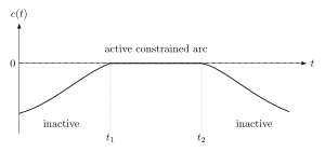
Figure 1:A state inequality constraint that is active on one interval.
This structure is an assumption. The true solution may have no constrained arc, one constrained arc, or several constrained arcs.
Constraint Derivatives
On the constrained arc,
Therefore, all total time derivatives must also vanish:
The total derivative is
Substituting the dynamics
gives
Order of a State Constraint
Assume that the control does not appear explicitly in
but appears explicitly in
Then the state constraint is said to have order .
Thus,
The highest derivative provides a control-dependent equality that can be used to determine the boundary control.
Tangency Conditions at Entry
At the entry time , the following conditions must hold:
These are the tangency conditions.
For a first-order constraint,
For a second-order constraint,
For a third-order constraint,
These conditions ensure that the trajectory joins the constraint boundary smoothly rather than crossing into the infeasible region.
Interior-Point Interpretation
The tangency conditions act as interior-point constraints:
where
Therefore, the constrained problem can be interpreted as a multiphase optimal control problem with an interior junction at .
The trajectory must satisfy:
unconstrained dynamics on ;
tangency conditions at ;
constrained dynamics on ;
exit or junction conditions at ;
unconstrained dynamics on .
Replacing the Inequality on the Active Arc
On the active arc, the original inequality
is replaced by the equality
The lower-order conditions remain satisfied as a consequence of the tangency conditions and the constrained dynamics.
In favorable cases, one can solve
for the boundary control:
Single and Multiple Constrained Arcs
The assumption of one active interval may be incorrect. The unconstrained solution may suggest several separate violations.
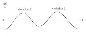
Figure 2:An unconstrained solution may violate a state inequality constraint over multiple intervals.
However, two unconstrained violations do not guarantee that the constrained optimal solution has two constrained arcs. Enforcing one arc may alter the trajectory enough to eliminate another violation.
Therefore, the active-set structure must be tested rather than blindly assumed.
Solve the Unconstrained Problem First
A practical indirect-method strategy is:
Solve the problem without the state inequality constraint.
Evaluate along the unconstrained trajectory.
If everywhere, the inequality is inactive.
If somewhere, identify approximate violation intervals.
Use these intervals to initialize candidate entry and exit times.
Solve constrained formulations with one or more candidate arcs.
Verify complementarity, tangency, and feasibility.
This strategy provides structural information before the difficult constrained boundary-value problem is attempted.
Risk of Assuming an Active Constraint Incorrectly
Suppose one assumes an active arc and imposes tangency and boundary-control conditions, even though the true optimum never activates the constraint.
The resulting solution is generally feasible for a more restrictive problem but is not the optimum of the original inequality-constrained problem. It is therefore suboptimal.
This illustrates a key principle:
Difficulty of Indirect Shooting
Without path constraints, an indirect method typically solves a two-point boundary-value problem consisting of:
state equations;
costate equations;
stationarity conditions;
endpoint boundary conditions;
transversality conditions.
A state inequality path constraint introduces:
unknown active intervals;
unknown entry and exit times;
interior tangency conditions;
boundary-control equations;
algebraic constraints on constrained arcs;
possible costate junction conditions.
The problem becomes a multiphase differential-algebraic boundary-value problem.
Transition to Direct Collocation
Direct collocation avoids explicit derivation of the constrained-arc structure in the problem formulation.
Consider the continuous optimal control problem
LGR/Radau Discretization
Using an -point Legendre–Gauss–Radau discretization, the cost is approximated by
The defect constraints are
More explicitly,
Endpoint constraints become
Discrete Path Constraints
The continuous path constraint
is enforced at the Radau points:
Equivalently,
No continuous-time path multiplier is explicitly introduced into the NLP formulation.
Why No Explicit Multiplier Is Added
The nonlinear program is written directly in terms of decision variables and constraints. The NLP solver introduces and estimates its own Lagrange multipliers internally as part of the Karush–Kuhn–Tucker conditions.
Therefore, the user provides:
the objective;
equality constraints;
inequality constraints;
variable bounds.
The solver determines which inequality constraints are active at the discrete optimum.
Major Advantage of Direct Collocation
Direct collocation does not require the user to specify:
whether a path constraint is active;
the number of constrained arcs;
the entry times;
the exit times;
tangency conditions in the NLP formulation.
The NLP solver identifies the discrete active set.
What the NLP Solver Actually Returns
The NLP solver returns a finite-dimensional decision vector,
not a continuous trajectory.
The quantities and are discrete samples. A reconstructed state and control must be produced by interpolation.
Therefore, satisfaction of a path constraint at the collocation points does not automatically imply satisfaction between those points.
Discrete Activity Does Not Prove a Continuous Constrained Arc
Suppose the NLP solution satisfies
at several neighboring Radau points.
This means only that those discrete constraints are active. It does not prove that
for every between them.
The reconstructed trajectory must be checked independently.
State Interpolation
For LGR collocation, the state approximation is uniquely defined by a Lagrange polynomial:
Thus, the state can be evaluated at dense points between the collocation nodes.
The corresponding physical time is
Control Interpolation
The control is represented only by its values at the collocation points:
Unlike the state, there is no unique control interpolation implied by the collocation derivation.
Possible choices include:
piecewise linear interpolation;
piecewise constant interpolation;
cubic splines;
local polynomial interpolation;
barycentric interpolation.
Different interpolation choices may produce different between-node behavior.
Hidden Constraint Violations
Even if
at every collocation point, an interpolated path may violate the constraint between nodes.
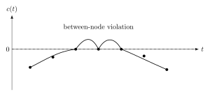
Figure 3:Discrete feasibility does not guarantee continuous feasibility.
This is a discretization error, not necessarily an NLP error.
Dense-Grid Verification
After solving the NLP:
reconstruct the state on a dense grid;
choose and document a control interpolation;
evaluate the path constraint on the dense grid;
compute the maximum violation;
compare it with a prescribed feasibility tolerance.
Define
A useful scalar metric is
Mesh Refinement
If the reconstructed solution violates the path constraint beyond tolerance, increase the mesh resolution.
Refinement may involve:
increasing the number of collocation points;
splitting the time interval into multiple mesh segments;
adding points near suspected entry and exit regions;
using adaptive -, -, or -refinement.
The process is repeated until the continuous residuals and violations are acceptably small.
Theory-Based Verification
Direct collocation simplifies the formulation, but theory remains essential for verifying the result.
For an apparently active state constraint, one should check:
whether the constraint is approximately zero on an interval;
whether the lower-order tangency conditions hold near entry;
whether the boundary control relation is approximately satisfied;
whether the constraint multiplier has the correct activity pattern;
whether the solution converges under mesh refinement.
NLP Multipliers and Continuous Path Multipliers
The NLP solver returns multipliers associated with the discrete path constraints. These can be interpreted as approximations of the continuous path multiplier after appropriate scaling.
On inactive points, the discrete multiplier should be near zero. On active points, it may be nonzero and should satisfy discrete complementarity.
For an upper-bound constraint
the discrete KKT conditions include
The sign depends on the NLP convention.
Equality Versus Inequality Constraints in an NLP
Defect constraints are equalities:
The NLP solver knows these must be active.
Path inequalities may be active or inactive:
The solver must determine which bounds bind at the solution.
This active-set determination may be performed through active-set methods, sequential quadratic programming, or interior-point methods.
Implementation Pattern
A typical MATLAB nonlinear-constraint function may be written as:
function [c, ceq] = constraints(z, data)

    [X, U, t0, tf] = unpackDecisionVector(z, data);

    t = ((tf - t0)/2) * data.tau + (tf + t0)/2;

    F = dynamics(X(:,1:data.N), U, t, data);

    defects = data.D * X.' ...
            - ((tf - t0)/2) * F.';

    boundary = endpointConstraints( ...
        X(:,1), t0, X(:,end), tf, data);

    path = pathFunctions( ...
        X(:,1:data.N), U, t, data);

    % Example upper-bound form: path <= pathMax
    cUpper = path - data.pathMax;

    % Example lower-bound form: path >= pathMin
    cLower = data.pathMin - path;

    c = [cUpper(:); cLower(:)];
    ceq = [defects(:); boundary(:)];
end
The path constraints are evaluated only at the collocation points inside the NLP. Dense-grid checking is performed after optimization.
Recommended Numerical Workflow
Formulate the continuous optimal control problem.
Identify all path constraints and their physical meaning.
Solve an unconstrained or relaxed problem first when useful.
Discretize the states and controls using collocation.
Add the path inequalities at all collocation points.
Solve the NLP using a scaled initial guess.
Inspect the solver status and KKT information.
Reconstruct state and control trajectories.
Evaluate dynamics residuals on a dense grid.
Evaluate path constraints on a dense grid.
Inspect active intervals and approximate tangency.
Refine the mesh and resolve.
Compare successive solutions and objective values.
Theory and Computation Must Work Together
A numerical solver does not understand optimal-control theory. It solves the finite-dimensional equations supplied by the user.
Therefore, obtaining a solver message such as “optimal solution found” is not enough. One must verify:
that the implemented equations represent the intended problem;
that the discretization is sufficiently accurate;
that path constraints hold between nodes;
that the result is consistent with necessary conditions;
that the solution is stable under mesh refinement.
Common Failure Modes
Incorrect Path Function
A sign error in the path constraint may reverse the feasible region.
Constraint Enforced at the Wrong Nodes
The control and dynamics may be defined only at the Radau points, while the state includes an additional terminal point. Indexing errors are common.
Assuming Discrete Feasibility Implies Continuous Feasibility
Interpolation can violate the constraint between nodes.
Inadequate Mesh Resolution
Entry and exit regions may be poorly resolved.
Poor Control Interpolation
A high-order global interpolation may oscillate and create artificial violations.
Blind Trust in Solver Output
An NLP solver can converge to a local optimum, a poorly scaled point, or the solution of incorrectly coded equations.
Summary
State inequality constraints may be inactive or active.
A constrained arc is an interval on which the state constraint is exactly active.
The order of the constraint is the number of derivatives required for the control to appear.
Entry tangency conditions require
On the active arc, the highest derivative condition determines the boundary control.
Indirect methods require assumptions about constrained-arc structure.
An incorrect active-set assumption may produce a suboptimal solution.
Direct collocation enforces path inequalities at discrete points.
The NLP solver determines the discrete active set.
Discrete feasibility does not guarantee continuous feasibility.
State and control interpolations must be checked on a dense grid.
Mesh refinement is required until constraint violations and residuals are acceptably small.
Continuous optimal-control theory is essential for validating direct numerical solutions.
Connection. Path-constrained trajectory optimization remains tied to a nominal initial condition; dynamic programming instead asks for optimal cost from every state and time.