The Principle of Optimality and the Hamilton–Jacobi–Bellman Equation

Earlier sections developed optimality conditions through the calculus of variations, Pontryagin’s minimum principle, and direct numerical methods. Those approaches typically produce an open-loop optimal trajectory for a specified initial condition and model.

Dynamic programming takes a different viewpoint. Instead of solving only for one optimal trajectory from one initial condition, it asks:

What is the minimum remaining cost from every possible state and every possible time?

The answer is encoded in the value function, also called the optimal cost-to-go. The partial differential equation satisfied by this function is the Hamilton–Jacobi–Bellman equation.

Open-Loop and Closed-Loop Optimal Control¶

An open-loop control is determined as a function of time:

\boldsymbol{u}^*(t).

(1)

It is computed for a particular initial state and a particular model. Once computed, the control does not explicitly change in response to deviations of the measured state.

A closed-loop control is a feedback law:

\boxed{ \boldsymbol{u}^*(t)=\boldsymbol{\pi}^*(\boldsymbol{x}(t),t). }

(2)

The current state is used to determine the control. Dynamic programming naturally generates this feedback form because it computes the optimal action for every state-time pair.

The Principle of Optimality¶

Suppose an optimal trajectory connects point $A$ to point $B$ . Let $D$ and $E$ be any two points lying on that trajectory.

Then the segment of the trajectory connecting $D$ to $E$ must itself be optimal for the subproblem that begins at $D$ and ends at $E$ .

A shorter geometric statement is:

\boxed{ \text{Every subarc of an optimal trajectory is optimal for its own endpoints.} }

(3)

What the Principle Does Not Mean¶

Suppose $C$ is not on the optimal trajectory from $A$ to $B$ . Even if the path from $A$ to $C$ is optimal and the path from $C$ to $B$ is optimal, the concatenated path

A\rightarrow C\rightarrow B

(4)

need not be optimal from $A$ to $B$ .

The principle of optimality applies only to subarcs of the original optimal path.

Geometric Illustration¶

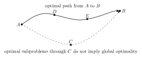
Figure 1:The principle of optimality applies to subarcs of the optimal trajectory.

Planning Backward and Executing Forward¶

Dynamic programming is based on a backward-planning idea:

Start from the terminal objective.
Determine the minimum remaining cost from states near the terminal time.
Continue backward in time.
Once the full policy is known, execute it forward in time.

This is often summarized by the statement:

Life is lived forward, but it is planned backward.

In control, one determines the optimal cost remaining from the current state to the terminal time. If the system deviates from the nominal path, the same value function provides the new optimal action from the new state.

Continuous-Time Optimal Control Problem¶

Consider

\begin{aligned} \dot{\boldsymbol{x}}(t) &= \boldsymbol{f}(\boldsymbol{x}(t),\boldsymbol{u}(t),t), \\ \boldsymbol{x}(t_0) &= \boldsymbol{x}_0, \end{aligned}

(5)

with Bolza cost

J = S(\boldsymbol{x}(t_f),t_f) + \int_{t_0}^{t_f} V(\boldsymbol{x}(t),\boldsymbol{u}(t),t)\,\mathrm{d} t.

(6)

The objective is to minimize $J$ over admissible controls.

The Cost-to-Go Function¶

Instead of starting only at $(\boldsymbol{x}_0,t_0)$ , define a problem beginning at an arbitrary state $\boldsymbol{x}$ and time $t$ :

J(\boldsymbol{x},t;\boldsymbol{u}) = S(\boldsymbol{x}(t_f),t_f) + \int_t^{t_f} V(\boldsymbol{x}(\tau),\boldsymbol{u}(\tau),\tau)\,\mathrm{d}\tau.

(7)

The optimal cost-to-go, or value function, is

\boxed{ J^*(\boldsymbol{x},t) = \min_{\boldsymbol{u}(\cdot)} \left[ S(\boldsymbol{x}(t_f),t_f) + \int_t^{t_f} V(\boldsymbol{x}(\tau),\boldsymbol{u}(\tau),\tau)\,\mathrm{d}\tau \right]. }

(8)

The terminal boundary condition is

\boxed{ J^*(\boldsymbol{x},t_f) = S(\boldsymbol{x},t_f). }

(9)

Interpretation of the Value Function¶

The value function answers the question:

If the system is currently at state $\boldsymbol{x}$ at time $t$ , what is the smallest possible cost that remains from now until the terminal time?

At the initial condition,

J^*(\boldsymbol{x}_0,t_0)

(10)

is the optimal value of the original problem.

Along an optimal trajectory,

J^*(\boldsymbol{x}^*(t),t)

(11)

decreases as cost is accumulated and eventually reaches the terminal cost.

Total Derivative Along the Optimal Trajectory¶

Along an optimal trajectory,

J^*=J^*(\boldsymbol{x}^*(t),t).

(12)

Its total derivative is

\frac{\,\mathrm{d} J^*}{\,\mathrm{d} t} = \frac{\partial J^*}{\partial t} + \left( \frac{\partial J^*}{\partial \boldsymbol{x}} \right)^{\mathsf{T}} \dot{\boldsymbol{x}}^*(t).

(13)

Because

J^*(\boldsymbol{x}^*(t),t) = S(\boldsymbol{x}^*(t_f),t_f) + \int_t^{t_f} V(\boldsymbol{x}^*(\tau),\boldsymbol{u}^*(\tau),\tau)\,\mathrm{d}\tau,

(14)

differentiating with respect to the lower integration limit gives

\frac{\,\mathrm{d} J^*}{\,\mathrm{d} t} = - V(\boldsymbol{x}^*(t),\boldsymbol{u}^*(t),t).

(15)

Therefore,

- V(\boldsymbol{x}^*,\boldsymbol{u}^*,t) = \frac{\partial J^*}{\partial t} + \left( \frac{\partial J^*}{\partial \boldsymbol{x}} \right)^{\mathsf{T}} \dot{\boldsymbol{x}}^*.

(16)

Substituting

\dot{\boldsymbol{x}}^* = \boldsymbol{f}(\boldsymbol{x}^*,\boldsymbol{u}^*,t)

(17)

yields

\boxed{ \frac{\partial J^*}{\partial t} + V(\boldsymbol{x}^*,\boldsymbol{u}^*,t) + \left( \frac{\partial J^*}{\partial \boldsymbol{x}} \right)^{\mathsf{T}} \boldsymbol{f}(\boldsymbol{x}^*,\boldsymbol{u}^*,t) = 0. }

(18)

Hamiltonian Form¶

Define the Hamiltonian

\mathcal{H}(\boldsymbol{x},\boldsymbol{u},\boldsymbol{p},t) = V(\boldsymbol{x},\boldsymbol{u},t) + \boldsymbol{p}^{\mathsf{T}}\boldsymbol{f}(\boldsymbol{x},\boldsymbol{u},t),

(19)

where

\boldsymbol{p} = \nabla_{\boldsymbol{x}}J^*(\boldsymbol{x},t).

(20)

Then, along the optimal trajectory,

\frac{\partial J^*}{\partial t} + \mathcal{H} \left( \boldsymbol{x}^*, \boldsymbol{u}^*, \nabla_{\boldsymbol{x}}J^*, t \right) = 0.

(21)

Because the control must minimize the Hamiltonian, the general HJB equation is

\boxed{ \frac{\partial J^*}{\partial t} + \min_{\boldsymbol{u}} \left[ V(\boldsymbol{x},\boldsymbol{u},t) + \left( \nabla_{\boldsymbol{x}}J^* \right)^{\mathsf{T}} \boldsymbol{f}(\boldsymbol{x},\boldsymbol{u},t) \right] = 0. }

(22)

The terminal condition is

\boxed{ J^*(\boldsymbol{x},t_f) = S(\boldsymbol{x},t_f). }

(23)

The Hamilton–Jacobi–Bellman Equation¶

The compact Hamiltonian form is

\boxed{ J_t^*(\boldsymbol{x},t) + \min_{\boldsymbol{u}} \mathcal{H} \left( \boldsymbol{x},\boldsymbol{u},\nabla_{\boldsymbol{x}}J^*,t \right) = 0. }

(24)

This is a nonlinear first-order partial differential equation with a terminal boundary condition.

Why the HJB Equation Is a Backward-Time Equation¶

The boundary condition is given at $t_f$ , not at $t_0$ :

J^*(\boldsymbol{x},t_f)=S(\boldsymbol{x},t_f).

(25)

Therefore, the HJB equation is integrated backward from the terminal time toward the initial time.

This matches the cost-to-go interpretation: one begins with the cost remaining at the end and works backward to determine the cost remaining at all earlier times.

Feedback Control from the HJB Equation¶

Once $J^*(\boldsymbol{x},t)$ is known, the optimal control is obtained from

\boxed{ \boldsymbol{u}^*(\boldsymbol{x},t) = \arg\min_{\boldsymbol{u}} \left[ V(\boldsymbol{x},\boldsymbol{u},t) + \left( \nabla_{\boldsymbol{x}}J^* \right)^{\mathsf{T}} \boldsymbol{f}(\boldsymbol{x},\boldsymbol{u},t) \right]. }

(26)

This is a state-feedback law.

The central advantage is that the solution is defined for all states in the domain, not merely along one nominal trajectory.

Relationship to the Costate¶

In Pontryagin’s minimum principle,

\boldsymbol{\lambda}^*(t)

(27)

is the costate.

In dynamic programming,

\nabla_{\boldsymbol{x}}J^*(\boldsymbol{x},t)

(28)

is the gradient of the value function.

Along an optimal trajectory,

\boxed{ \boldsymbol{\lambda}^*(t) = \nabla_{\boldsymbol{x}}J^*(\boldsymbol{x}^*(t),t). }

(29)

Thus, the costate is the gradient of the optimal cost-to-go evaluated along the optimal path.

Connection to the Costate Equation¶

Differentiate

\boldsymbol{\lambda}^*(t) = \nabla_{\boldsymbol{x}}J^*(\boldsymbol{x}^*(t),t)

(30)

with respect to time:

\dot{\boldsymbol{\lambda}}^*(t) = \frac{\,\mathrm{d}}{\,\mathrm{d} t} \nabla_{\boldsymbol{x}}J^*(\boldsymbol{x}^*(t),t).

(31)

The HJB equation implies the same costate dynamics as Pontryagin’s minimum principle:

\boxed{ \dot{\boldsymbol{\lambda}}^* = - \frac{\partial \mathcal{H}}{\partial \boldsymbol{x}}. }

(32)

Therefore, the HJB equation and the minimum principle are consistent descriptions of optimality.

Why HJB Is More General Than a Single Open-Loop Solution¶

Pontryagin’s principle typically produces an extremal trajectory for a specified initial state.

The HJB equation produces the full value function

J^*(\boldsymbol{x},t),

(33)

which contains the optimal cost from every state and time.

Consequently, the HJB equation can generate feedback control even after disturbances or modeling errors move the system away from the nominal trajectory.

Replanning Interpretation¶

Suppose the nominal trajectory is interrupted by an unexpected change. The current state becomes

\boldsymbol{x}_{\mathrm{new}}.

(34)

One does not need to return to the original initial condition. Instead, the optimal policy evaluates

\boldsymbol{u}^*(\boldsymbol{x}_{\mathrm{new}},t)

(35)

and continues optimally from the current state.

This is the mathematical version of replanning a route after encountering a road closure.

Computational Challenge¶

The HJB equation is a PDE in state and time. If the state dimension is $n_x$ , then the value function is defined over an $(n_x+1)$ -dimensional domain.

The computational burden grows rapidly with $n_x$ . This is known as the curse of dimensionality.

This makes direct solution of the HJB equation impractical for many high-dimensional systems.

Introductory Scalar Linear–Quadratic Example¶

Consider

\boxed{ J = \frac{1}{2}x^2(t_f) + \frac{1}{2} \int_0^{t_f} \left[ x^2(t)+u^2(t) \right]\,\mathrm{d} t }

(36)

subject to

\boxed{ \dot{x}(t) = -2x(t)+u(t), \qquad x(0)=x_0. }

(37)

The running cost is

V(x,u,t) = \frac{1}{2}x^2 + \frac{1}{2}u^2.

(38)

The terminal cost is

S(x(t_f),t_f) = \frac{1}{2}x^2(t_f).

(39)

The dynamics are

f(x,u,t) = -2x+u.

(40)

Hamiltonian for the Example¶

The HJB Hamiltonian is

\mathcal{H}(x,u,J_x,t) = \frac{1}{2}x^2 + \frac{1}{2}u^2 + J_x(-2x+u).

(41)

The minimizing control satisfies

\frac{\partial \mathcal{H}}{\partial u} = u+J_x = 0.

(42)

Therefore,

\boxed{ u^*(x,t) = - J_x^*(x,t). }

(43)

Substituting into the Hamiltonian gives

\begin{aligned} \mathcal{H}^* &= \frac{1}{2}x^2 + \frac{1}{2}(J_x^*)^2 + J_x^* \left( -2x-J_x^* \right) \\ &= \frac{1}{2}x^2 - \frac{1}{2}(J_x^*)^2 - 2xJ_x^*. \end{aligned}

(44)

Hence, the HJB equation is

\boxed{ J_t^* + \frac{1}{2}x^2 - \frac{1}{2}(J_x^*)^2 - 2xJ_x^* = 0. }

(45)

The terminal condition is

\boxed{ J^*(x,t_f) = \frac{1}{2}x^2. }

(46)

Quadratic Value-Function Ansatz¶

Because the dynamics are linear and the cost is quadratic, assume

\boxed{ J^*(x,t) = \frac{1}{2}P(t)x^2. }

(47)

The terminal condition gives

\frac{1}{2}P(t_f)x^2 = \frac{1}{2}x^2,

(48)

\boxed{ P(t_f)=1. }

(49)

The derivatives are

\begin{aligned} J_x^* &= P(t)x, \\ J_t^* &= \frac{1}{2}\dot{P}(t)x^2. \end{aligned}

(50)

Optimal Feedback Law¶

Using

u^* = - J_x^*,

(51)

the optimal control becomes

\boxed{ u^*(t) = - P(t)x^*(t). }

(52)

This is a time-varying linear state-feedback law.

The feedback gain is

K(t)=P(t).

(53)

Riccati Differential Equation¶

Substitute the quadratic ansatz into the HJB equation:

\frac{1}{2}\dot{P}x^2 + \frac{1}{2}x^2 - \frac{1}{2}P^2x^2 - 2Px^2 = 0.

(54)

For nonzero $x$ , divide by $\frac{1}{2}x^2$ :

\dot{P} + 1 - P^2 - 4P = 0.

(55)

Therefore,

\boxed{ \dot{P} = P^2+4P-1, \qquad P(t_f)=1. }

(56)

This differential equation is integrated backward in time.

Closed-Loop State Dynamics¶

Substituting

u^*=-P(t)x

(57)

into the system dynamics gives

\boxed{ \dot{x}^*(t) = -\left[2+P(t)\right]x^*(t). }

(58)

Once $P(t)$ is found backward in time, the optimal state can be propagated forward from

x(0)=x_0.

(59)

Backward Planning and Forward Execution¶

The solution procedure has two stages:

Integrate the Riccati equation backward from

P(t_f)=1.

(60)

Integrate the closed-loop state equation forward from

x(0)=x_0.

(61)

This is the precise mathematical realization of planning backward and executing forward.

Numerical MATLAB Template¶

tf = 5;

% Backward Riccati equation
riccati = @(t,P) P.^2 + 4*P - 1;

% Integrate backward from P(tf) = 1
[tP, P] = ode45(riccati, [tf 0], 1);

% Reverse arrays for interpolation in increasing time
tP = flipud(tP);
P  = flipud(P);

Pfun = @(t) interp1(tP, P, t, 'pchip');

% Initial state
x0 = 1;

% Closed-loop dynamics
closedLoop = @(t,x) -(2 + Pfun(t))*x;

% Integrate state forward
[tx, x] = ode45(closedLoop, [0 tf], x0);

% Optimal control
u = -arrayfun(Pfun, tx).*x;

Verification Checks¶

For the scalar example, verify:

$P(t_f)=1$ ;
the Riccati residual is small;
$u^*(t)=-P(t)x^*(t)$ ;
the state satisfies

\dot{x}^*=-2x^*+u^*;

(62)

the HJB residual is small;
the value function decreases consistently with the accumulated running cost.

HJB Residual¶

For an approximate value function $\widehat{J}(x,t)$ and control $\widehat{u}(x,t)$ , define

R_{\mathrm{HJB}} = \widehat{J}_t + V(x,\widehat{u},t) + \widehat{J}_x f(x,\widehat{u},t).

(63)

A high-quality approximation should satisfy

\boxed{ R_{\mathrm{HJB}}\approx 0. }

(64)

Comparison with Pontryagin’s Minimum Principle¶

For this example, the Hamiltonian in the minimum principle is

\mathcal{H} = \frac{1}{2}x^2 + \frac{1}{2}u^2 + \lambda(-2x+u).

(65)

Stationarity gives

u^*=-\lambda.

(66)

Dynamic programming gives

u^*=-J_x^*.

(67)

Therefore,

\boxed{ \lambda(t) = J_x^*(x^*(t),t) = P(t)x^*(t). }

(68)

The two methods produce the same optimal control.

Summary¶

The principle of optimality states that every subarc of an optimal trajectory is itself optimal.
The value function is the minimum remaining cost from a state-time pair.
The terminal condition is specified at $t_f$ .
The HJB equation is solved backward in time.
The general continuous-time HJB equation is

J_t^* + \min_{\boldsymbol{u}} \left[ V + (\nabla_{\boldsymbol{x}}J^*)^{\mathsf{T}}\boldsymbol{f} \right] = 0.

(69)

The optimal feedback law is obtained by minimizing the HJB Hamiltonian.
Along the optimal trajectory,

\boldsymbol{\lambda}^*=\nabla_{\boldsymbol{x}}J^*.

(70)

Dynamic programming produces a feedback law rather than only one open-loop trajectory.
The HJB equation suffers from the curse of dimensionality.
For linear systems with quadratic costs, a quadratic value function leads to a Riccati differential equation.
The scalar example produces

u^*(t)=-P(t)x^*(t).

(71)

Connection. Applying the HJB equation to finite-horizon LQR shows how a quadratic value function turns a nonlinear PDE into a matrix differential equation.