Neighboring Optimal Control
Suppose an optimal state, control, and costate trajectory have already been computed:
x ∗ ( t ) , u ∗ ( t ) , λ ∗ ( t ) . \boldsymbol{x}^*(t),\qquad
\boldsymbol{u}^*(t),\qquad
\boldsymbol{\lambda}^*(t). x ∗ ( t ) , u ∗ ( t ) , λ ∗ ( t ) . During implementation, disturbances, model mismatch, sensor error, and imperfect actuation may move the system away from this nominal optimal trajectory. One response is to solve the original nonlinear optimal control problem again. However, repeated nonlinear optimization may be too computationally expensive for real-time implementation.
Neighboring optimal control provides a local alternative. It constructs an approximately optimal correction near the nominal solution by:
linearizing the dynamics about the nominal optimal trajectory;
approximating the cost to second order;
solving the resulting time-varying linear-quadratic problem;
applying a feedback correction to the nominal control.
Nominal Optimal Control Problem ¶ Consider the fixed-time problem
min u ( ⋅ ) J = Φ ( x ( t f ) ) + ∫ t 0 t f L ( x ( t ) , u ( t ) ) d t \min_{\boldsymbol{u}(\cdot)}
J
=
\Phi\bigl(\boldsymbol{x}(t_f)\bigr)
+
\int_{t_0}^{t_f}
L\bigl(\boldsymbol{x}(t),\boldsymbol{u}(t)\bigr)\,\mathrm{d} t u ( ⋅ ) min J = Φ ( x ( t f ) ) + ∫ t 0 t f L ( x ( t ) , u ( t ) ) d t subject to
x ˙ ( t ) = f ( x ( t ) , u ( t ) ) , x ( t 0 ) = x 0 . \begin{aligned}
\dot{\boldsymbol{x}}(t)
&=
\boldsymbol{f}\bigl(\boldsymbol{x}(t),\boldsymbol{u}(t)\bigr),\\
\boldsymbol{x}(t_0)
&=
\boldsymbol{x}_0.
\end{aligned} x ˙ ( t ) x ( t 0 ) = f ( x ( t ) , u ( t ) ) , = x 0 . For clarity, explicit time dependence, path constraints, and free-final-time terms are omitted. The neighboring-optimal-control idea extends to more general formulations.
Assume
( x ∗ ( t ) , u ∗ ( t ) , λ ∗ ( t ) ) \left(
\boldsymbol{x}^*(t),
\boldsymbol{u}^*(t),
\boldsymbol{\lambda}^*(t)
\right) ( x ∗ ( t ) , u ∗ ( t ) , λ ∗ ( t ) ) satisfies the first-order necessary conditions.
Neighboring Trajectories ¶ Define perturbed trajectories:
x ( t ) = x ∗ ( t ) + δ x ( t ) , u ( t ) = u ∗ ( t ) + δ u ( t ) , λ ( t ) = λ ∗ ( t ) + δ λ ( t ) . \begin{aligned}
\boldsymbol{x}(t)
&=
\boldsymbol{x}^*(t)+\delta\boldsymbol{x}(t),\\
\boldsymbol{u}(t)
&=
\boldsymbol{u}^*(t)+\delta\boldsymbol{u}(t),\\
\boldsymbol{\lambda}(t)
&=
\boldsymbol{\lambda}^*(t)+\delta\boldsymbol{\lambda}(t).
\end{aligned} x ( t ) u ( t ) λ ( t ) = x ∗ ( t ) + δ x ( t ) , = u ∗ ( t ) + δ u ( t ) , = λ ∗ ( t ) + δ λ ( t ) . The quantities
δ x ( t ) , δ u ( t ) , δ λ ( t ) \delta\boldsymbol{x}(t),\qquad
\delta\boldsymbol{u}(t),\qquad
\delta\boldsymbol{\lambda}(t) δ x ( t ) , δ u ( t ) , δ λ ( t ) are neighboring variations.
If the actual initial condition differs from the nominal one,
x ( t 0 ) = x 0 + δ x 0 , \boldsymbol{x}(t_0)
=
\boldsymbol{x}_0+\delta\boldsymbol{x}_0, x ( t 0 ) = x 0 + δ x 0 , then
δ x ( t 0 ) = δ x 0 . \boxed{
\delta\boldsymbol{x}(t_0)=\delta\boldsymbol{x}_0.
} δ x ( t 0 ) = δ x 0 . Why a Second-Order Cost Approximation Is Required ¶ At an optimal solution, the first variation of the cost vanishes:
Therefore, a first-order cost approximation cannot distinguish neighboring directions. The leading nonzero local change in cost is generally the second variation:
J ≈ J ∗ + 1 2 δ 2 J . J
\approx
J^*
+
\frac{1}{2}\delta^2J. J ≈ J ∗ + 2 1 δ 2 J . This is analogous to a static minimization problem.
Static Second-Order Expansion ¶ For a scalar function g ( z ) g(\boldsymbol{z}) g ( z )
g ( z ∗ + Δ z ) ≈ g ( z ∗ ) + g z ( z ∗ ) Δ z + 1 2 Δ z T g z z ( z ∗ ) Δ z . \begin{aligned}
g(\boldsymbol{z}^*+\Delta\boldsymbol{z})
\approx{}&
g(\boldsymbol{z}^*)
+
g_{\boldsymbol{z}}(\boldsymbol{z}^*)\Delta\boldsymbol{z}
\nonumber\\
&+
\frac{1}{2}
\Delta\boldsymbol{z}^{\mathsf{T}}
g_{\boldsymbol{z}\boldsymbol{z}}(\boldsymbol{z}^*)
\Delta\boldsymbol{z}.
\end{aligned} g ( z ∗ + Δ z ) ≈ g ( z ∗ ) + g z ( z ∗ ) Δ z + 2 1 Δ z T g z z ( z ∗ ) Δ z . At a local minimum,
g z ( z ∗ ) = 0 , g_{\boldsymbol{z}}(\boldsymbol{z}^*)=\boldsymbol{0}, g z ( z ∗ ) = 0 , so
g ( z ∗ + Δ z ) ≈ g ( z ∗ ) + 1 2 Δ z T g z z ( z ∗ ) Δ z . g(\boldsymbol{z}^*+\Delta\boldsymbol{z})
\approx
g(\boldsymbol{z}^*)
+
\frac{1}{2}
\Delta\boldsymbol{z}^{\mathsf{T}}
g_{\boldsymbol{z}\boldsymbol{z}}(\boldsymbol{z}^*)
\Delta\boldsymbol{z}. g ( z ∗ + Δ z ) ≈ g ( z ∗ ) + 2 1 Δ z T g z z ( z ∗ ) Δ z . The neighboring optimal control derivation follows the same principle for functions of time.
Second Variation of the Cost Functional ¶ The terminal contribution is
1 2 δ x T ( t f ) Φ x x ∗ δ x ( t f ) , \frac{1}{2}
\delta\boldsymbol{x}^{\mathsf{T}}(t_f)
\Phi_{\boldsymbol{x}\boldsymbol{x}}^*
\delta\boldsymbol{x}(t_f), 2 1 δ x T ( t f ) Φ x x ∗ δ x ( t f ) , where
Φ x x ∗ = ∂ 2 Φ ∂ x 2 ∣ x ∗ ( t f ) . \Phi_{\boldsymbol{x}\boldsymbol{x}}^*
=
\left.
\frac{\partial^2\Phi}{\partial\boldsymbol{x}^2}
\right|_{\boldsymbol{x}^*(t_f)}. Φ x x ∗ = ∂ x 2 ∂ 2 Φ ∣ ∣ x ∗ ( t f ) . The running-cost contribution is
1 2 ∫ t 0 t f [ δ x δ u ] T [ L x x ∗ L x u ∗ L u x ∗ L u u ∗ ] [ δ x δ u ] d t . \frac{1}{2}
\int_{t_0}^{t_f}
\begin{bmatrix}
\delta\boldsymbol{x}\\
\delta\boldsymbol{u}
\end{bmatrix}^{\mathsf{T}}
\begin{bmatrix}
L_{\boldsymbol{x}\boldsymbol{x}}^* & L_{\boldsymbol{x}\boldsymbol{u}}^*\\
L_{\boldsymbol{u}\boldsymbol{x}}^* & L_{\boldsymbol{u}\boldsymbol{u}}^*
\end{bmatrix}
\begin{bmatrix}
\delta\boldsymbol{x}\\
\delta\boldsymbol{u}
\end{bmatrix}
\,\mathrm{d} t. 2 1 ∫ t 0 t f [ δ x δ u ] T [ L x x ∗ L u x ∗ L x u ∗ L u u ∗ ] [ δ x δ u ] d t . Define
P f = Φ x x ∗ , Q ( t ) = L x x ∗ , M ( t ) = L x u ∗ , R ( t ) = L u u ∗ . \begin{aligned}
\boldsymbol{P}_f
&=
\Phi_{\boldsymbol{x}\boldsymbol{x}}^*,\\
\boldsymbol{Q}(t)
&=
L_{\boldsymbol{x}\boldsymbol{x}}^*,\\
\boldsymbol{M}(t)
&=
L_{\boldsymbol{x}\boldsymbol{u}}^*,\\
\boldsymbol{R}(t)
&=
L_{\boldsymbol{u}\boldsymbol{u}}^*.
\end{aligned} P f Q ( t ) M ( t ) R ( t ) = Φ x x ∗ , = L x x ∗ , = L x u ∗ , = L u u ∗ . Then
δ 2 J = 1 2 δ x T ( t f ) P f δ x ( t f ) + 1 2 ∫ t 0 t f [ δ x T Q δ x + 2 δ x T M δ u + δ u T R δ u ] d t . \begin{aligned}
\delta^2J
={}&
\frac{1}{2}
\delta\boldsymbol{x}^{\mathsf{T}}(t_f)
\boldsymbol{P}_f
\delta\boldsymbol{x}(t_f)
\nonumber\\
&+
\frac{1}{2}
\int_{t_0}^{t_f}
\left[
\delta\boldsymbol{x}^{\mathsf{T}}\boldsymbol{Q}\delta\boldsymbol{x}
+
2\delta\boldsymbol{x}^{\mathsf{T}}\boldsymbol{M}\delta\boldsymbol{u}
+
\delta\boldsymbol{u}^{\mathsf{T}}\boldsymbol{R}\delta\boldsymbol{u}
\right]\,\mathrm{d} t.
\end{aligned} δ 2 J = 2 1 δ x T ( t f ) P f δ x ( t f ) + 2 1 ∫ t 0 t f [ δ x T Q δ x + 2 δ x T M δ u + δ u T R δ u ] d t . Linearized Neighboring Dynamics ¶ Expand the nonlinear dynamics:
x ˙ ∗ + δ x ˙ ≈ f ( x ∗ , u ∗ ) + f x ∗ δ x + f u ∗ δ u . \begin{aligned}
\dot{\boldsymbol{x}}^*+\delta\dot{\boldsymbol{x}}
\approx{}&
\boldsymbol{f}(\boldsymbol{x}^*,\boldsymbol{u}^*)
+
\boldsymbol{f}_{\boldsymbol{x}}^*\delta\boldsymbol{x}
+
\boldsymbol{f}_{\boldsymbol{u}}^*\delta\boldsymbol{u}.
\end{aligned} x ˙ ∗ + δ x ˙ ≈ f ( x ∗ , u ∗ ) + f x ∗ δ x + f u ∗ δ u . Because
x ˙ ∗ = f ( x ∗ , u ∗ ) , \dot{\boldsymbol{x}}^*
=
\boldsymbol{f}(\boldsymbol{x}^*,\boldsymbol{u}^*), x ˙ ∗ = f ( x ∗ , u ∗ ) , the nominal terms cancel.
Define
F ( t ) = ∂ f ∂ x ∣ ( x ∗ , u ∗ ) , G ( t ) = ∂ f ∂ u ∣ ( x ∗ , u ∗ ) . \begin{aligned}
\boldsymbol{F}(t)
&=
\left.
\frac{\partial\boldsymbol{f}}{\partial\boldsymbol{x}}
\right|_{(\boldsymbol{x}^*,\boldsymbol{u}^*)},\\
\boldsymbol{G}(t)
&=
\left.
\frac{\partial\boldsymbol{f}}{\partial\boldsymbol{u}}
\right|_{(\boldsymbol{x}^*,\boldsymbol{u}^*)}.
\end{aligned} F ( t ) G ( t ) = ∂ x ∂ f ∣ ∣ ( x ∗ , u ∗ ) , = ∂ u ∂ f ∣ ∣ ( x ∗ , u ∗ ) . The neighboring dynamics are
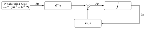
δ x ˙ = F ( t ) δ x + G ( t ) δ u . \boxed{
\delta\dot{\boldsymbol{x}}
=
\boldsymbol{F}(t)\delta\boldsymbol{x}
+
\boldsymbol{G}(t)\delta\boldsymbol{u}.
} δ x ˙ = F ( t ) δ x + G ( t ) δ u . Neighboring Optimal Control Problem ¶ The local correction problem is therefore
min δ u ( ⋅ ) δ 2 J \min_{\delta\boldsymbol{u}(\cdot)}
\delta^2J δ u ( ⋅ ) min δ 2 J subject to
δ x ˙ = F δ x + G δ u , δ x ( t 0 ) = δ x 0 . \begin{aligned}
\delta\dot{\boldsymbol{x}}
&=
\boldsymbol{F}\delta\boldsymbol{x}+\boldsymbol{G}\delta\boldsymbol{u},\\
\delta\boldsymbol{x}(t_0)
&=
\delta\boldsymbol{x}_0.
\end{aligned} δ x ˙ δ x ( t 0 ) = F δ x + G δ u , = δ x 0 . This is a finite-horizon, time-varying linear-quadratic optimal control problem with state–control coupling.
Neighboring Hamiltonian ¶ The Hamiltonian for the neighboring problem is
H N = 1 2 δ x T Q δ x + δ x T M δ u + 1 2 δ u T R δ u + δ λ T ( F δ x + G δ u ) . \begin{aligned}
\mathcal{H}_N
={}&
\frac{1}{2}
\delta\boldsymbol{x}^{\mathsf{T}}\boldsymbol{Q}\delta\boldsymbol{x}
+
\delta\boldsymbol{x}^{\mathsf{T}}\boldsymbol{M}\delta\boldsymbol{u}
+
\frac{1}{2}
\delta\boldsymbol{u}^{\mathsf{T}}\boldsymbol{R}\delta\boldsymbol{u}
\nonumber\\
&+
\delta\boldsymbol{\lambda}^{\mathsf{T}}
\left(
\boldsymbol{F}\delta\boldsymbol{x}+\boldsymbol{G}\delta\boldsymbol{u}
\right).
\end{aligned} H N = 2 1 δ x T Q δ x + δ x T M δ u + 2 1 δ u T R δ u + δ λ T ( F δ x + G δ u ) . Neighboring Costate Equation ¶ The costate dynamics satisfy
δ λ ˙ = − ∂ H N ∂ δ x . \delta\dot{\boldsymbol{\lambda}}
=
-\frac{\partial\mathcal{H}_N}{\partial\delta\boldsymbol{x}}. δ λ ˙ = − ∂ δ x ∂ H N . Hence,
δ λ ˙ = − Q δ x − M δ u − F T δ λ . \boxed{
\delta\dot{\boldsymbol{\lambda}}
=
-\boldsymbol{Q}\delta\boldsymbol{x}
-\boldsymbol{M}\delta\boldsymbol{u}
-\boldsymbol{F}^{\mathsf{T}}\delta\boldsymbol{\lambda}.
} δ λ ˙ = − Q δ x − M δ u − F T δ λ . The terminal boundary condition is
δ λ ( t f ) = P f δ x ( t f ) . \boxed{
\delta\boldsymbol{\lambda}(t_f)
=
\boldsymbol{P}_f\delta\boldsymbol{x}(t_f).
} δ λ ( t f ) = P f δ x ( t f ) . Stationarity and Neighboring Optimal Control ¶ The stationarity condition is
∂ H N ∂ δ u = 0 . \frac{\partial\mathcal{H}_N}{\partial\delta\boldsymbol{u}}
=
\boldsymbol{0}. ∂ δ u ∂ H N = 0 . Therefore,
M T δ x + R δ u + G T δ λ = 0 . \boldsymbol{M}^{\mathsf{T}}\delta\boldsymbol{x}
+
\boldsymbol{R}\delta\boldsymbol{u}
+
\boldsymbol{G}^{\mathsf{T}}\delta\boldsymbol{\lambda}
=
\boldsymbol{0}. M T δ x + R δ u + G T δ λ = 0 . Assuming R \boldsymbol{R} R
δ u ∗ = − R − 1 ( M T δ x + G T δ λ ) . \boxed{
\delta\boldsymbol{u}^*
=
-\boldsymbol{R}^{-1}
\left(
\boldsymbol{M}^{\mathsf{T}}\delta\boldsymbol{x}
+
\boldsymbol{G}^{\mathsf{T}}\delta\boldsymbol{\lambda}
\right).
} δ u ∗ = − R − 1 ( M T δ x + G T δ λ ) . Coupled State–Costate System ¶ Substituting the stationarity condition into the state dynamics gives
δ x ˙ = ( F − G R − 1 M T ) δ x − G R − 1 G T δ λ . \boxed{
\delta\dot{\boldsymbol{x}}
=
\left(
\boldsymbol{F}
-
\boldsymbol{G}\boldsymbol{R}^{-1}\boldsymbol{M}^{\mathsf{T}}
\right)\delta\boldsymbol{x}
-
\boldsymbol{G}\boldsymbol{R}^{-1}\boldsymbol{G}^{\mathsf{T}}\delta\boldsymbol{\lambda}.
} δ x ˙ = ( F − G R − 1 M T ) δ x − G R − 1 G T δ λ . Substitution into the costate equation gives
δ λ ˙ = − ( Q − M R − 1 M T ) δ x − ( F T − M R − 1 G T ) δ λ . \boxed{
\delta\dot{\boldsymbol{\lambda}}
=
-
\left(
\boldsymbol{Q}
-
\boldsymbol{M}\boldsymbol{R}^{-1}\boldsymbol{M}^{\mathsf{T}}
\right)\delta\boldsymbol{x}
-
\left(
\boldsymbol{F}^{\mathsf{T}}
-
\boldsymbol{M}\boldsymbol{R}^{-1}\boldsymbol{G}^{\mathsf{T}}
\right)\delta\boldsymbol{\lambda}.
} δ λ ˙ = − ( Q − M R − 1 M T ) δ x − ( F T − M R − 1 G T ) δ λ . The boundary conditions are split:
δ x ( t 0 ) = δ x 0 , δ λ ( t f ) = P f δ x ( t f ) . \begin{aligned}
\delta\boldsymbol{x}(t_0)&=\delta\boldsymbol{x}_0,\\
\delta\boldsymbol{\lambda}(t_f)&=\boldsymbol{P}_f\delta\boldsymbol{x}(t_f).
\end{aligned} δ x ( t 0 ) δ λ ( t f ) = δ x 0 , = P f δ x ( t f ) . Thus, the neighboring necessary conditions form a linear two-point boundary-value problem.
Assume a linear relationship between neighboring costate and neighboring state:
δ λ ( t ) = P ( t ) δ x ( t ) . \boxed{
\delta\boldsymbol{\lambda}(t)=\boldsymbol{P}(t)\delta\boldsymbol{x}(t).
} δ λ ( t ) = P ( t ) δ x ( t ) . Differentiating,
δ λ ˙ = P ˙ δ x + P δ x ˙ . \delta\dot{\boldsymbol{\lambda}}
=
\dot{\boldsymbol{P}}\delta\boldsymbol{x}
+
\boldsymbol{P}\delta\dot{\boldsymbol{x}}. δ λ ˙ = P ˙ δ x + P δ x ˙ . Substituting the state and costate equations and requiring the result to hold for all δ x \delta\boldsymbol{x} δ x
Generalized Riccati Differential Equation ¶ The resulting equation is
P ˙ = − Q + M R − 1 M T − ( F T − M R − 1 G T ) P − P ( F − G R − 1 M T ) + P G R − 1 G T P . \begin{aligned}
\dot{\boldsymbol{P}}
={}&
-\boldsymbol{Q}
+
\boldsymbol{M}\boldsymbol{R}^{-1}\boldsymbol{M}^{\mathsf{T}}
\nonumber\\
&-
\left(
\boldsymbol{F}^{\mathsf{T}}
-
\boldsymbol{M}\boldsymbol{R}^{-1}\boldsymbol{G}^{\mathsf{T}}
\right)\boldsymbol{P}
\nonumber\\
&-
\boldsymbol{P}
\left(
\boldsymbol{F}
-
\boldsymbol{G}\boldsymbol{R}^{-1}\boldsymbol{M}^{\mathsf{T}}
\right)
\nonumber\\
&+
\boldsymbol{P}\boldsymbol{G}\boldsymbol{R}^{-1}\boldsymbol{G}^{\mathsf{T}}\boldsymbol{P}.
\end{aligned} P ˙ = − Q + M R − 1 M T − ( F T − M R − 1 G T ) P − P ( F − G R − 1 M T ) + P G R − 1 G T P . Equivalently,
− P ˙ = Q + F T P + P F − ( P G + M ) R − 1 ( G T P + M T ) . \begin{aligned}
-\dot{\boldsymbol{P}}
={}&
\boldsymbol{Q}
+
\boldsymbol{F}^{\mathsf{T}}\boldsymbol{P}
+
\boldsymbol{P}\boldsymbol{F}
\nonumber\\
&-
\left(
\boldsymbol{P}\boldsymbol{G}+\boldsymbol{M}
\right)
\boldsymbol{R}^{-1}
\left(
\boldsymbol{G}^{\mathsf{T}}\boldsymbol{P}+\boldsymbol{M}^{\mathsf{T}}
\right).
\end{aligned} − P ˙ = Q + F T P + P F − ( P G + M ) R − 1 ( G T P + M T ) . The terminal condition is
P ( t f ) = P f . \boxed{
\boldsymbol{P}(t_f)=\boldsymbol{P}_f.
} P ( t f ) = P f . This equation is integrated backward from t f t_f t f t 0 t_0 t 0
Neighboring Optimal Feedback Law ¶ Using
δ λ = P δ x \delta\boldsymbol{\lambda}=\boldsymbol{P}\delta\boldsymbol{x} δ λ = P δ x in the stationarity condition,
δ u ∗ = − R − 1 ( M T + G T P ) δ x . \begin{aligned}
\delta\boldsymbol{u}^*
&=
-\boldsymbol{R}^{-1}
\left(
\boldsymbol{M}^{\mathsf{T}}
+
\boldsymbol{G}^{\mathsf{T}}\boldsymbol{P}
\right)\delta\boldsymbol{x}.
\end{aligned} δ u ∗ = − R − 1 ( M T + G T P ) δ x . Define the time-varying gain
K ( t ) = R − 1 ( t ) [ M T ( t ) + G T ( t ) P ( t ) ] . \boxed{
\boldsymbol{K}(t)
=
\boldsymbol{R}^{-1}(t)
\left[
\boldsymbol{M}^{\mathsf{T}}(t)
+
\boldsymbol{G}^{\mathsf{T}}(t)\boldsymbol{P}(t)
\right].
} K ( t ) = R − 1 ( t ) [ M T ( t ) + G T ( t ) P ( t ) ] . Then
δ u ∗ ( t ) = − K ( t ) δ x ( t ) . \boxed{
\delta\boldsymbol{u}^*(t)
=
-\boldsymbol{K}(t)\delta\boldsymbol{x}(t).
} δ u ∗ ( t ) = − K ( t ) δ x ( t ) . The implemented control becomes
u ( t ) = u ∗ ( t ) − K ( t ) [ x ( t ) − x ∗ ( t ) ] . \boxed{
\boldsymbol{u}(t)
=
\boldsymbol{u}^*(t)
-
\boldsymbol{K}(t)
\left[
\boldsymbol{x}(t)-\boldsymbol{x}^*(t)
\right].
} u ( t ) = u ∗ ( t ) − K ( t ) [ x ( t ) − x ∗ ( t ) ] . This is a trajectory-tracking feedback law centered on the nonlinear optimal solution.
Closed-Loop Neighboring Dynamics ¶ Substituting the feedback law into the linearized dynamics gives
δ x ˙ = [ F − G K ] δ x . \delta\dot{\boldsymbol{x}}
=
\left[
\boldsymbol{F}
-
\boldsymbol{G}\boldsymbol{K}
\right]\delta\boldsymbol{x}. δ x ˙ = [ F − G K ] δ x . Hence,
δ x ˙ = [ F − G R − 1 ( M T + G T P ) ] δ x . \boxed{
\delta\dot{\boldsymbol{x}}
=
\left[
\boldsymbol{F}
-
\boldsymbol{G}\boldsymbol{R}^{-1}
\left(
\boldsymbol{M}^{\mathsf{T}}
+
\boldsymbol{G}^{\mathsf{T}}\boldsymbol{P}
\right)
\right]\delta\boldsymbol{x}.
} δ x ˙ = [ F − G R − 1 ( M T + G T P ) ] δ x . Block-Diagram Interpretation ¶ Figure 1: Neighboring optimal feedback around the nominal trajectory.
Interpretation of the Cross Matrix M \boldsymbol{M} M ¶ The matrix
M = L x u ∗ \boldsymbol{M}
=
L_{\boldsymbol{x}\boldsymbol{u}}^* M = L x u ∗ captures local coupling between state and control variations in the running cost.
When M = 0 \boldsymbol{M}=\boldsymbol{0} M = 0
− P ˙ = Q + F T P + P F − P G R − 1 G T P . -\dot{\boldsymbol{P}}
=
\boldsymbol{Q}
+
\boldsymbol{F}^{\mathsf{T}}\boldsymbol{P}
+
\boldsymbol{P}\boldsymbol{F}
-
\boldsymbol{P}\boldsymbol{G}\boldsymbol{R}^{-1}\boldsymbol{G}^{\mathsf{T}}\boldsymbol{P}. − P ˙ = Q + F T P + P F − P G R − 1 G T P . The feedback gain becomes
K = R − 1 G T P . \boldsymbol{K}
=
\boldsymbol{R}^{-1}\boldsymbol{G}^{\mathsf{T}}\boldsymbol{P}. K = R − 1 G T P . Completing the Square ¶ The running quadratic form can be written as
δ x T Q δ x + 2 δ x T M δ u + δ u T R δ u = ( δ u + R − 1 M T δ x ) T R ( δ u + R − 1 M T δ x ) + δ x T ( Q − M R − 1 M T ) δ x . \begin{aligned}
&\delta\boldsymbol{x}^{\mathsf{T}}\boldsymbol{Q}\delta\boldsymbol{x}
+
2\delta\boldsymbol{x}^{\mathsf{T}}\boldsymbol{M}\delta\boldsymbol{u}
+
\delta\boldsymbol{u}^{\mathsf{T}}\boldsymbol{R}\delta\boldsymbol{u}
\nonumber\\
={}&
\left(
\delta\boldsymbol{u}+\boldsymbol{R}^{-1}\boldsymbol{M}^{\mathsf{T}}\delta\boldsymbol{x}
\right)^{\mathsf{T}}
\boldsymbol{R}
\left(
\delta\boldsymbol{u}+\boldsymbol{R}^{-1}\boldsymbol{M}^{\mathsf{T}}\delta\boldsymbol{x}
\right)
\nonumber\\
&+
\delta\boldsymbol{x}^{\mathsf{T}}
\left(
\boldsymbol{Q}
-
\boldsymbol{M}\boldsymbol{R}^{-1}\boldsymbol{M}^{\mathsf{T}}
\right)
\delta\boldsymbol{x}.
\end{aligned} = δ x T Q δ x + 2 δ x T M δ u + δ u T R δ u ( δ u + R − 1 M T δ x ) T R ( δ u + R − 1 M T δ x ) + δ x T ( Q − M R − 1 M T ) δ x . This shows why the effective state penalty is
Q e f f = Q − M R − 1 M T . \boxed{
\boldsymbol{Q}_{\mathrm{eff}}
=
\boldsymbol{Q}
-
\boldsymbol{M}\boldsymbol{R}^{-1}\boldsymbol{M}^{\mathsf{T}}.
} Q eff = Q − M R − 1 M T . Conditions for a Well-Defined Neighboring Controller ¶ Several assumptions are important.
Positive Definiteness of R \boldsymbol{R} R ¶ Because the feedback law requires R − 1 \boldsymbol{R}^{-1} R − 1
R ( t ) ≻ 0 \boxed{
\boldsymbol{R}(t)\succ\boldsymbol{0}
} R ( t ) ≻ 0 is commonly imposed.
Positive semidefiniteness is insufficient when R \boldsymbol{R} R
State Penalty ¶ Typically,
Q ( t ) ⪰ 0 , P f ⪰ 0 . \boldsymbol{Q}(t)\succeq\boldsymbol{0},
\qquad
\boldsymbol{P}_f\succeq\boldsymbol{0}. Q ( t ) ⪰ 0 , P f ⪰ 0 . With a cross term, a stronger convexity condition may be expressed through the block Hessian:
[ Q M M T R ] ⪰ 0 . \begin{bmatrix}
\boldsymbol{Q} & \boldsymbol{M}\\
\boldsymbol{M}^{\mathsf{T}} & \boldsymbol{R}
\end{bmatrix}
\succeq\boldsymbol{0}. [ Q M T M R ] ⪰ 0 . Controllability or Stabilizability ¶ The pair
( F ( t ) , G ( t ) ) (\boldsymbol{F}(t),\boldsymbol{G}(t)) ( F ( t ) , G ( t )) should be controllable or at least stabilizable over the interval.
Otherwise, some deviations cannot be corrected.
Observability or Detectability ¶ The state penalty and system dynamics should provide adequate detectability. In standard LQR language, an appropriate pair related to
( F , Q 1 / 2 ) (\boldsymbol{F},\boldsymbol{Q}^{1/2}) ( F , Q 1/2 ) should be detectable.
Small Perturbations ¶ The method relies on local approximations:
f ( x , u ) ≈ f ∗ + F δ x + G δ u , J ≈ J ∗ + 1 2 δ 2 J . \begin{aligned}
\boldsymbol{f}(\boldsymbol{x},\boldsymbol{u})
&\approx
\boldsymbol{f}^*
+
\boldsymbol{F}\delta\boldsymbol{x}
+
\boldsymbol{G}\delta\boldsymbol{u},\\
J
&\approx
J^*
+
\frac{1}{2}\delta^2J.
\end{aligned} f ( x , u ) J ≈ f ∗ + F δ x + G δ u , ≈ J ∗ + 2 1 δ 2 J . Therefore,
∥ δ x ∥ , ∥ δ u ∥ \|\delta\boldsymbol{x}\|,
\qquad
\|\delta\boldsymbol{u}\| ∥ δ x ∥ , ∥ δ u ∥ must remain sufficiently small.
Neighboring Control versus Reoptimization ¶ Two correction strategies are possible after a disturbance.
Neighboring-Control Correction ¶ Use
δ u = − K δ x . \delta\boldsymbol{u}=-\boldsymbol{K}\delta\boldsymbol{x}. δ u = − K δ x . Advantages include:
rapid online evaluation;
no repeated nonlinear optimization;
locally optimal correction;
simple feedback implementation.
The limitation is local validity.
Full Reoptimization ¶ Resolve the nonlinear optimal control problem from the new state.
Advantages include:
handles large deviations;
incorporates nonlinearities directly;
can update active constraints and trajectory structure.
The limitation is computational cost.
Offline and Online Computation ¶ A practical implementation can separate computation into two stages.
Offline Stage ¶ solve the nonlinear optimal control problem;
store x ∗ ( t ) \boldsymbol{x}^*(t) x ∗ ( t ) u ∗ ( t ) \boldsymbol{u}^*(t) u ∗ ( t )
compute F \boldsymbol{F} F G \boldsymbol{G} G Q \boldsymbol{Q} Q M \boldsymbol{M} M R \boldsymbol{R} R
integrate the Riccati equation backward;
store P ( t ) \boldsymbol{P}(t) P ( t ) K ( t ) \boldsymbol{K}(t) K ( t )
Online Stage ¶ At each control update:
estimate the current state x ^ ( t ) \hat{\boldsymbol{x}}(t) x ^ ( t )
compute
δ x ( t ) = x ^ ( t ) − x ∗ ( t ) ; \delta\boldsymbol{x}(t)=\hat{\boldsymbol{x}}(t)-\boldsymbol{x}^*(t); δ x ( t ) = x ^ ( t ) − x ∗ ( t ) ; evaluate the stored gain K ( t ) \boldsymbol{K}(t) K ( t )
compute
δ u = − K ( t ) δ x ; \delta\boldsymbol{u}=-\boldsymbol{K}(t)\delta\boldsymbol{x}; δ u = − K ( t ) δ x ; apply
u = u ∗ + δ u . \boldsymbol{u}=\boldsymbol{u}^*+\delta\boldsymbol{u}. u = u ∗ + δ u . The Riccati equation need not be integrated online if the nominal trajectory and gain schedule are known in advance.
Parallel-Processor Interpretation ¶ In some architectures, one processor may compute or update the Riccati solution while another applies the real-time feedback law. However, for a fixed nominal trajectory, it is often preferable to compute the gain schedule offline and store it.
Parallel online computation may be useful when:
the nominal trajectory changes;
the final time changes;
model parameters are updated;
gains must be recomputed adaptively.
Relation to Time-Varying LQR ¶ Neighboring optimal control is closely related to trajectory linearization followed by finite-horizon time-varying LQR.
The distinction is that its weighting matrices are not chosen arbitrarily. They arise from the second derivatives of the original nonlinear optimal control problem:
Q = L x x ∗ , M = L x u ∗ , R = L u u ∗ , P f = Φ x x ∗ . \begin{aligned}
\boldsymbol{Q}&=L_{\boldsymbol{x}\boldsymbol{x}}^*,\\
\boldsymbol{M}&=L_{\boldsymbol{x}\boldsymbol{u}}^*,\\
\boldsymbol{R}&=L_{\boldsymbol{u}\boldsymbol{u}}^*,\\
\boldsymbol{P}_f&=\Phi_{\boldsymbol{x}\boldsymbol{x}}^*.
\end{aligned} Q M R P f = L x x ∗ , = L x u ∗ , = L u u ∗ , = Φ x x ∗ . Thus, the local controller is tied directly to the original nonlinear objective.
Connection to Differential Dynamic Programming ¶ Neighboring optimal control and differential dynamic programming share the use of:
local linearization of dynamics;
second-order cost information;
backward Riccati-like recursions;
local feedback policies around a nominal trajectory.
Differential dynamic programming goes further by iteratively updating the nominal trajectory and repeating the local approximation.
Implementation Workflow ¶ A complete workflow is:
solve the nominal nonlinear optimal control problem;
verify the nominal state, control, and constraints;
compute first derivatives of the dynamics;
compute second derivatives of terminal and running costs;
construct the neighboring LQ problem;
check symmetry and definiteness;
solve the generalized Riccati equation backward;
construct the gain schedule;
simulate the perturbed nonlinear system;
compare neighboring feedback with open-loop execution;
determine the perturbation range over which the approximation remains accurate.
MATLAB Skeleton ¶ t = linspace(t0,tf,N);
% F(:,:,k), G(:,:,k), Q(:,:,k), M(:,:,k), and R(:,:,k)
% are evaluated along x_star(t), u_star(t).
% Integrate P backward from P(tf) = Pf.
P = zeros(nx,nx,N);
P(:,:,N) = Pf;
for k = N:-1:2
dt = t(k)-t(k-1);
Fk = F(:,:,k);
Gk = G(:,:,k);
Qk = Q(:,:,k);
Mk = M(:,:,k);
Rk = R(:,:,k);
Pk = P(:,:,k);
Pdot = -Qk ...
+ Mk*(Rk\Mk') ...
- (Fk' - Mk*(Rk\Gk'))*Pk ...
- Pk*(Fk - Gk*(Rk\Mk')) ...
+ Pk*Gk*(Rk\Gk')*Pk;
% Backward Euler illustration.
P(:,:,k-1) = Pk - dt*Pdot;
end
% Gain schedule.
K = zeros(nu,nx,N);
for k = 1:N
K(:,:,k) = R(:,:,k) \ ...
(M(:,:,k)' + G(:,:,k)'*P(:,:,k));
end
% Online correction:
% delta_x = x_measured - x_star;
% delta_u = -K(:,:,k)*delta_x;
% u = u_star + delta_u;For high-quality computation, use a suitable ODE solver rather than the illustrative backward-Euler update.
Verification Tests ¶ A neighboring optimal controller should be tested for:
zero correction on the nominal trajectory;
correct Riccati terminal condition;
symmetry of P ( t ) \boldsymbol{P}(t) P ( t )
positive definiteness of R ( t ) \boldsymbol{R}(t) R ( t )
bounded feedback gains;
closed-loop decay of small perturbations;
performance under nonlinear dynamics;
sensitivity to state-estimation error;
actuator limits;
failure under large perturbations.
Common Errors ¶ retaining only first-order cost terms even though δ J = 0 \delta J=0 δ J = 0
omitting the mixed Hessian M \boldsymbol{M} M
using the wrong Riccati terminal condition;
integrating the Riccati equation forward instead of backward;
confusing δ u \delta\boldsymbol{u} δ u u \boldsymbol{u} u
applying the local controller too far from the nominal trajectory;
assuming R − 1 \boldsymbol{R}^{-1} R − 1
linearizing about a nonoptimal or dynamically inconsistent trajectory.
Summary ¶ Neighboring optimal control begins with a nominal nonlinear optimal trajectory.
The state, control, and costate are perturbed around that trajectory.
The first variation vanishes on the optimal solution.
Therefore, the cost must be retained to second order.
The dynamics are linearized to first order.
The result is a time-varying LQ problem with a state–control cross term.
The neighboring Hamiltonian produces linear state and costate equations.
A Riccati transformation converts the two-point boundary-value problem into a backward matrix differential equation.
The optimal correction is a time-varying feedback law.
The total control is the nominal optimal control plus the neighboring correction.
The method is appropriate for small perturbations.
Large deviations generally require nonlinear reoptimization.