Inequality Path Constraints, Complementarity, and Constrained Arcs

This section develops the necessary conditions for inequality path constraints. It introduces active and inactive constraints, complementary slackness, control inequality constraints, state inequality constraints, constrained arcs, and entry conditions. The emphasis is on the theoretical structure that must hold along an optimal trajectory.

Control Inequality Path Constraints¶

Consider

\boxed{ \boldsymbol{c}(\boldsymbol{u},t)\leq \boldsymbol{0}. }

(1)

Introduce the augmented Hamiltonian

\mathcal{H}_A = \mathcal{H} - \boldsymbol{\mu}^{\mathsf{T}}\boldsymbol{c}.

(2)

The multiplier is time varying. The stationarity condition is

\boxed{ \frac{\partial \mathcal{H}}{\partial \boldsymbol{u}} - \left( \frac{\partial \boldsymbol{c}}{\partial \boldsymbol{u}} \right)^{\mathsf{T}}\boldsymbol{\mu} = \boldsymbol{0}. }

(3)

Because the constraint is independent of the state,

\dot{\boldsymbol{\lambda}} = - \frac{\partial \mathcal{H}}{\partial \boldsymbol{x}}.

(4)

Active and Inactive Constraints¶

For a scalar constraint $c(\boldsymbol{u},t)\leq 0$ :

The constraint is inactive if $c<0$ .
The constraint is active if $c=0$ .

If the unconstrained optimal control already satisfies the bound strictly, then the constraint has no effect on the solution.

Complementary Slackness¶

The multiplier and constraint must satisfy

\boxed{ \boldsymbol{\mu}^{\mathsf{T}}\boldsymbol{c}=\boldsymbol{0}. }

(5)

With the sign convention

\mathcal{H}_A=\mathcal{H}-\boldsymbol{\mu}^{\mathsf{T}}\boldsymbol{c}, \qquad \boldsymbol{c}\leq\boldsymbol{0},

(6)

the multiplier satisfies

\boxed{ \boldsymbol{\mu}\leq\boldsymbol{0}. }

(7)

Componentwise,

\mu_i c_i=0, \qquad \mu_i\leq 0, \qquad c_i\leq 0.

(8)

Thus:

\begin{aligned} c_i<0 &\Longrightarrow \mu_i=0, \\ c_i=0 &\Longrightarrow \mu_i\leq 0. \end{aligned}

(9)

Interpretation of the Multiplier¶

The path multiplier represents the local sensitivity of the optimal cost to relaxation of the constraint. An inactive constraint has zero sensitivity. An active constraint may have a nonzero multiplier.

The sign depends on the convention used in the augmented Hamiltonian. A different sign convention changes the sign restriction but not the underlying complementarity structure.

Complete Conditions for a Control Inequality¶

For

\boldsymbol{c}(\boldsymbol{u},t)\leq\boldsymbol{0},

(10)

the necessary conditions include

\begin{aligned} \dot{\boldsymbol{x}} &= \frac{\partial\mathcal{H}_A}{\partial\boldsymbol{\lambda}}, \\ \dot{\boldsymbol{\lambda}} &= - \frac{\partial\mathcal{H}_A}{\partial\boldsymbol{x}}, \\ \frac{\partial\mathcal{H}_A}{\partial\boldsymbol{u}} &= \boldsymbol{0}, \\ \boldsymbol{c} &\leq \boldsymbol{0}, \\ \boldsymbol{\mu} &\leq \boldsymbol{0}, \\ \boldsymbol{\mu}^{\mathsf{T}}\boldsymbol{c} &= 0. \end{aligned}

(11)

These are supplemented by endpoint conditions and transversality conditions.

State Inequality Path Constraints¶

Now consider

\boxed{ \boldsymbol{c}(\boldsymbol{x},t)\leq\boldsymbol{0}. }

(12)

This case is more difficult for two reasons:

the constraint does not directly appear in the control stationarity equation;
the times at which the constraint becomes active are generally unknown.

The augmented Hamiltonian is

\mathcal{H}_A = \mathcal{H}-\boldsymbol{\mu}^{\mathsf{T}}\boldsymbol{c}.

(13)

The costate equation is

\boxed{ \dot{\boldsymbol{\lambda}} = - \frac{\partial \mathcal{H}}{\partial \boldsymbol{x}} + \left( \frac{\partial \boldsymbol{c}}{\partial \boldsymbol{x}} \right)^{\mathsf{T}}\boldsymbol{\mu}. }

(14)

The ordinary stationarity equation remains

\frac{\partial \mathcal{H}}{\partial \boldsymbol{u}} = \boldsymbol{0}

(15)

until the state constraint is differentiated enough times for the control to appear.

Unconstrained and Constrained Arcs¶

An optimal trajectory may consist of:

an unconstrained arc, where $\boldsymbol{c}<\boldsymbol{0}$ ;
a constrained arc, where $\boldsymbol{c}=\boldsymbol{0}$ ;
a second unconstrained arc after leaving the boundary.

A qualitative scalar picture is shown below.

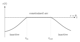
Figure 1:An inequality constraint with inactive and constrained arcs.

Unknown Junction Times¶

The entry time $t_{\mathrm{in}}$ and exit time $t_{\mathrm{out}}$ are generally unknown. They become additional unknowns in an indirect formulation.

This is one reason state inequality constraints are significantly harder than control bounds.

Constraint Order on a Constrained Arc¶

Suppose the state constraint has order $q$ . Define

\boldsymbol{c}^{(0)}=\boldsymbol{c}.

(16)

Differentiate until the control appears:

\begin{aligned} \boldsymbol{c}^{(0)}(\boldsymbol{x},t)&=\boldsymbol{0},\\ \boldsymbol{c}^{(1)}(\boldsymbol{x},t)&=\boldsymbol{0},\\ &\vdots\\ \boldsymbol{c}^{(q-1)}(\boldsymbol{x},t)&=\boldsymbol{0},\\ \boldsymbol{c}^{(q)}(\boldsymbol{x},\boldsymbol{u},t)&=\boldsymbol{0}. \end{aligned}

(17)

These equalities hold on the active constrained arc.

Entry Conditions¶

At the entry point, continuity and tangency require

\boxed{ \boldsymbol{c}^{(j)}(t_{\mathrm{in}})=\boldsymbol{0}, \qquad j=0,\ldots,q-1. }

(18)

For a first-order scalar state constraint,

c(t_{\mathrm{in}})=0.

(19)

For a second-order state constraint,

c(t_{\mathrm{in}})=0, \qquad \dot{c}(t_{\mathrm{in}})=0.

(20)

These conditions ensure tangential contact with the constraint boundary rather than crossing into the infeasible region.

Tangency Interpretation¶

At the moment a smooth trajectory reaches an active state boundary, it must become tangent to that boundary.

For a scalar state constraint:

c<0

(21)

on the unconstrained side and

c=0

(22)

on the constrained arc.

If $\dot{c}$ were positive at entry for a constraint $c\leq 0$ , the trajectory would immediately enter the infeasible region. Therefore, the appropriate tangency conditions must hold.

Control on the Constrained Arc¶

Once the state constraint has been differentiated until the control appears, the highest-order relation

\boldsymbol{c}^{(q)}(\boldsymbol{x},\boldsymbol{u},t)=\boldsymbol{0}

(23)

can often be solved for the boundary control:

\boxed{ \boldsymbol{u}=\boldsymbol{u}_{\mathrm{boundary}}(\boldsymbol{x},t). }

(24)

This control keeps the state exactly on the active boundary.

Multiplier Behavior¶

On inactive arcs:

\boldsymbol{\mu}=\boldsymbol{0}.

(25)

On active arcs:

\boldsymbol{c}=\boldsymbol{0}, \qquad \boldsymbol{\mu}\leq\boldsymbol{0}.

(26)

The multiplier may change at entry and exit points. Depending on the order and regularity of the state constraint, the costate may exhibit junction conditions or jumps. A full derivation of those jump conditions belongs to the continuation of the state-constraint theory.

Why Inequality State Constraints Are Difficult¶

They require simultaneous determination of:

the unconstrained solution;
the constrained solution;
the entry time;
the exit time;
the boundary control;
the path multiplier;
the junction conditions.

Therefore, the resulting indirect problem is a multiphase boundary-value problem with unknown switching times.

Direct Transcription Interpretation¶

In direct collocation, inequality path constraints are imposed at the discretization points:

\boldsymbol{c}_{\min} \leq \boldsymbol{c}(\boldsymbol{X}_i,\boldsymbol{U}_i,t_i) \leq \boldsymbol{c}_{\max}.

(27)

The NLP solver determines which constraints are active. The corresponding NLP multipliers approximate the continuous path multipliers.

This is one reason direct methods are often preferred for complicated path-constrained problems.

Control Bounds as a Special Case¶

A box constraint

\boldsymbol{u}_{\min} \leq \boldsymbol{u}(t) \leq \boldsymbol{u}_{\max}

(28)

can be represented by

\begin{aligned} \boldsymbol{u}-\boldsymbol{u}_{\max}&\leq\boldsymbol{0},\\ \boldsymbol{u}_{\min}-\boldsymbol{u}&\leq\boldsymbol{0}. \end{aligned}

(29)

Each side has its own multiplier and complementary-slackness condition.

State Bounds as a Special Case¶

Similarly,

\boldsymbol{x}_{\min} \leq \boldsymbol{x}(t) \leq \boldsymbol{x}_{\max}

(30)

is represented by two sets of state inequality constraints.

Unlike control bounds, state bounds may have nonzero order and can generate constrained arcs.

Summary¶

Inequality path constraints may be active or inactive.
Inactive constraints have zero multiplier.
Active constraints satisfy the boundary equality and may have nonzero multiplier.
Complementary slackness is

\boldsymbol{\mu}^{\mathsf{T}}\boldsymbol{c}=0.

(31)

Under the convention $\mathcal{H}_A=\mathcal{H}-\boldsymbol{\mu}^{\mathsf{T}}\boldsymbol{c}$ with $\boldsymbol{c}\leq 0$ , one has $\boldsymbol{\mu}\leq 0$ .
Control inequalities directly modify stationarity.
State inequalities must be differentiated until the control appears.
Active state constraints generate constrained arcs.
Entry conditions enforce contact and tangency.
Unknown entry and exit times make indirect formulations difficult.
Direct collocation handles active-set identification through the NLP solver.

Connection. State inequalities are especially subtle because the control affects them through the dynamics and their active intervals are not known in advance.