Natural Boundary Conditions and the Structure of Optimal Control Problems
The calculus of variations produces two distinct kinds of necessary conditions:
differential equations governing the trajectory in the interior of the time interval;
boundary or transversality conditions governing behavior at the endpoints.
The endpoint conditions depend directly on which endpoint quantities are fixed and which are free. A small change in the problem statement can therefore produce a significantly different boundary condition.
This section first revisits the free-final-time case through a worked example. It then derives the natural boundary condition for a free terminal state at fixed final time. The chapter also develops standard vector-derivative notation and introduces the principal ingredients of a general optimal control problem: dynamics, boundary conditions, static parameters, controls, and performance indices.
Review: Fixed Terminal State and Free Terminal Time ¶ Consider
J [ x , t f ] = ∫ t 0 t f L ( x , x ˙ , t ) d t , J[x,t_f]
=
\int_{t_0}^{t_f}
L(x,\dot{x},t)\,\mathrm{d} t, J [ x , t f ] = ∫ t 0 t f L ( x , x ˙ , t ) d t , with
x ( t 0 ) = x 0 , x ( t f ) = x f , \begin{aligned}
x(t_0)&=x_0,\\
x(t_f)&=x_f,
\end{aligned} x ( t 0 ) x ( t f ) = x 0 , = x f , where t 0 t_0 t 0 x 0 x_0 x 0 x f x_f x f t f t_f t f
The necessary conditions are
∂ L ∂ x − d d t ( ∂ L ∂ x ˙ ) = 0 \frac{\partial L}{\partial x}
-
\frac{\,\mathrm{d}}{\,\mathrm{d} t}
\left(
\frac{\partial L}{\partial\dot{x}}
\right)
=
0 ∂ x ∂ L − d t d ( ∂ x ˙ ∂ L ) = 0 and
[ L − x ˙ ∂ L ∂ x ˙ ] t f = 0. \left[
L
-
\dot{x}
\frac{\partial L}{\partial\dot{x}}
\right]_{t_f}
=
0. [ L − x ˙ ∂ x ˙ ∂ L ] t f = 0. The first equation governs the interior trajectory. The second supplies the missing boundary condition associated with the free final time.
Worked Example: A Free-Final-Time Variational Problem ¶ Consider
J [ x , t f ] = ∫ 1 t f [ 2 x ( t ) + 1 2 x ˙ 2 ( t ) ] d t , J[x,t_f]
=
\int_1^{t_f}
\left[
2x(t)
+
\frac{1}{2}\dot{x}^2(t)
\right]\,\mathrm{d} t, J [ x , t f ] = ∫ 1 t f [ 2 x ( t ) + 2 1 x ˙ 2 ( t ) ] d t , subject to
x ( 1 ) = 4 , x ( t f ) = 4 , t f > 1. x(1)=4,
\qquad
x(t_f)=4,
\qquad
t_f>1. x ( 1 ) = 4 , x ( t f ) = 4 , t f > 1. The integrand is
L ( x , x ˙ , t ) = 2 x + 1 2 x ˙ 2 . L(x,\dot{x},t)
=
2x+\frac{1}{2}\dot{x}^2. L ( x , x ˙ , t ) = 2 x + 2 1 x ˙ 2 . Euler–Lagrange equation ¶ We have
∂ L ∂ x = 2 \frac{\partial L}{\partial x}=2 ∂ x ∂ L = 2 and
∂ L ∂ x ˙ = x ˙ . \frac{\partial L}{\partial\dot{x}}
=
\dot{x}. ∂ x ˙ ∂ L = x ˙ . Thus,
d d t ( ∂ L ∂ x ˙ ) = x ¨ . \frac{\,\mathrm{d}}{\,\mathrm{d} t}
\left(
\frac{\partial L}{\partial\dot{x}}
\right)
=
\ddot{x}. d t d ( ∂ x ˙ ∂ L ) = x ¨ . The Euler–Lagrange equation gives
2 − x ¨ = 0 , 2-\ddot{x}=0, 2 − x ¨ = 0 , or
x ¨ = 2 . \boxed{
\ddot{x}=2
}. x ¨ = 2 . Integrating twice yields
x ( t ) = t 2 + c 1 t + c 2 . x(t)
=
t^2+c_1t+c_2. x ( t ) = t 2 + c 1 t + c 2 . Initial boundary condition ¶ Using x ( 1 ) = 4 x(1)=4 x ( 1 ) = 4
1 + c 1 + c 2 = 4 , 1+c_1+c_2=4, 1 + c 1 + c 2 = 4 , so
c 1 + c 2 = 3. c_1+c_2=3. c 1 + c 2 = 3. Free-final-time condition ¶ The transversality condition is
[ L − x ˙ ∂ L ∂ x ˙ ] t f = 0. \left[
L
-
\dot{x}
\frac{\partial L}{\partial\dot{x}}
\right]_{t_f}
=
0. [ L − x ˙ ∂ x ˙ ∂ L ] t f = 0. Since
∂ L ∂ x ˙ = x ˙ , \frac{\partial L}{\partial\dot{x}}
=
\dot{x}, ∂ x ˙ ∂ L = x ˙ , we obtain
0 = [ 2 x + 1 2 x ˙ 2 − x ˙ 2 ] t f = [ 2 x − 1 2 x ˙ 2 ] t f . \begin{aligned}
0
&=
\left[
2x+\frac{1}{2}\dot{x}^2-\dot{x}^2
\right]_{t_f}
\nonumber\\
&=
\left[
2x-\frac{1}{2}\dot{x}^2
\right]_{t_f}.
\end{aligned} 0 = [ 2 x + 2 1 x ˙ 2 − x ˙ 2 ] t f = [ 2 x − 2 1 x ˙ 2 ] t f . Using the terminal-state condition x ( t f ) = 4 x(t_f)=4 x ( t f ) = 4
8 − 1 2 x ˙ 2 ( t f ) = 0 , 8-\frac{1}{2}\dot{x}^2(t_f)=0, 8 − 2 1 x ˙ 2 ( t f ) = 0 , which implies
x ˙ 2 ( t f ) = 16. \dot{x}^2(t_f)=16. x ˙ 2 ( t f ) = 16. Therefore,
x ˙ ( t f ) = ± 4. \dot{x}(t_f)=\pm4. x ˙ ( t f ) = ± 4. From (13)
x ˙ ( t ) = 2 t + c 1 . \dot{x}(t)=2t+c_1. x ˙ ( t ) = 2 t + c 1 . Combining this with
x ( t f ) = t f 2 + c 1 t f + c 2 = 4 x(t_f)=t_f^2+c_1t_f+c_2=4 x ( t f ) = t f 2 + c 1 t f + c 2 = 4 and (15) t f > 1 t_f>1 t f > 1
t f = 5 \boxed{
t_f=5
} t f = 5 with
c 1 = − 6 , c 2 = 9. c_1=-6,
\qquad
c_2=9. c 1 = − 6 , c 2 = 9. Hence,
x ∗ ( t ) = t 2 − 6 t + 9 . \boxed{
x^*(t)
=
t^2-6t+9
}. x ∗ ( t ) = t 2 − 6 t + 9 . A direct check gives
x ∗ ( 1 ) = 4 , x ∗ ( 5 ) = 4 , x ˙ ∗ ( 5 ) = 4. \begin{aligned}
x^*(1)&=4,\\
x^*(5)&=4,\\
\dot{x}^*(5)&=4.
\end{aligned} x ∗ ( 1 ) x ∗ ( 5 ) x ˙ ∗ ( 5 ) = 4 , = 4 , = 4. Free Terminal State with Fixed Final Time ¶ Now consider
J [ x ] = ∫ t 0 t f L ( x , x ˙ , t ) d t , J[x]
=
\int_{t_0}^{t_f}
L(x,\dot{x},t)\,\mathrm{d} t, J [ x ] = ∫ t 0 t f L ( x , x ˙ , t ) d t , subject to
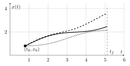
x ( t 0 ) = x 0 , x(t_0)=x_0, x ( t 0 ) = x 0 , where t 0 t_0 t 0 t f t_f t f x ( t f ) x(t_f) x ( t f )
The endpoint configuration is shown conceptually in Figure 1
Figure 1: When t f t_f t f x ( t f ) x(t_f) x ( t f ) t = t f t=t_f t = t f
Derivation of the Natural Boundary Condition ¶ Because the endpoint times are fixed, variation of the functional gives
δ J = ∫ t 0 t f δ L d t . \delta J
=
\int_{t_0}^{t_f}
\delta L\,\mathrm{d} t. δ J = ∫ t 0 t f δ L d t . To first order,
δ L = ∂ L ∂ x δ x + ∂ L ∂ x ˙ δ x ˙ . \delta L
=
\frac{\partial L}{\partial x}\delta x
+
\frac{\partial L}{\partial\dot{x}}
\delta\dot{x}. δ L = ∂ x ∂ L δ x + ∂ x ˙ ∂ L δ x ˙ . Thus,
δ J = ∫ t 0 t f [ ∂ L ∂ x δ x + ∂ L ∂ x ˙ δ x ˙ ] d t . \delta J
=
\int_{t_0}^{t_f}
\left[
\frac{\partial L}{\partial x}\delta x
+
\frac{\partial L}{\partial\dot{x}}
\delta\dot{x}
\right]\,\mathrm{d} t. δ J = ∫ t 0 t f [ ∂ x ∂ L δ x + ∂ x ˙ ∂ L δ x ˙ ] d t . Using
δ x ˙ = d d t δ x \delta\dot{x}
=
\frac{\,\mathrm{d}}{\,\mathrm{d} t}\delta x δ x ˙ = d t d δ x and integrating by parts,
δ J = ∂ L ∂ x ˙ δ x ∣ t 0 t f + ∫ t 0 t f [ ∂ L ∂ x − d d t ( ∂ L ∂ x ˙ ) ] δ x d t . \begin{aligned}
\delta J
&=
\left.
\frac{\partial L}{\partial\dot{x}}
\delta x
\right|_{t_0}^{t_f}
\nonumber\\
&\quad
+
\int_{t_0}^{t_f}
\left[
\frac{\partial L}{\partial x}
-
\frac{\,\mathrm{d}}{\,\mathrm{d} t}
\left(
\frac{\partial L}{\partial\dot{x}}
\right)
\right]
\delta x\,\mathrm{d} t.
\end{aligned} δ J = ∂ x ˙ ∂ L δ x ∣ ∣ t 0 t f + ∫ t 0 t f [ ∂ x ∂ L − d t d ( ∂ x ˙ ∂ L ) ] δ x d t . Since the initial state is fixed,
δ x ( t 0 ) = 0. \delta x(t_0)=0. δ x ( t 0 ) = 0. Since t f t_f t f
δ t f = 0. \delta t_f=0. δ t f = 0. The endpoint identity
δ x f = δ x ( t f ) + x ˙ ( t f ) δ t f \delta x_f
=
\delta x(t_f)
+
\dot{x}(t_f)\delta t_f δ x f = δ x ( t f ) + x ˙ ( t f ) δ t f therefore reduces to
δ x f = δ x ( t f ) . \delta x_f
=
\delta x(t_f). δ x f = δ x ( t f ) . Because the terminal state is free,
δ x ( t f ) \delta x(t_f) δ x ( t f ) is arbitrary and generally nonzero.
Equation (34)
δ J = ∂ L ∂ x ˙ ∣ t f δ x ( t f ) + ∫ t 0 t f [ ∂ L ∂ x − d d t ( ∂ L ∂ x ˙ ) ] δ x d t . \begin{aligned}
\delta J
&=
\left.
\frac{\partial L}{\partial\dot{x}}
\right|_{t_f}
\delta x(t_f)
\nonumber\\
&\quad
+
\int_{t_0}^{t_f}
\left[
\frac{\partial L}{\partial x}
-
\frac{\,\mathrm{d}}{\,\mathrm{d} t}
\left(
\frac{\partial L}{\partial\dot{x}}
\right)
\right]
\delta x\,\mathrm{d} t.
\end{aligned} δ J = ∂ x ˙ ∂ L ∣ ∣ t f δ x ( t f ) + ∫ t 0 t f [ ∂ x ∂ L − d t d ( ∂ x ˙ ∂ L ) ] δ x d t . Since the interior variation and terminal variation are independent, the necessary conditions are
∂ L ∂ x − d d t ( ∂ L ∂ x ˙ ) = 0 \boxed{
\frac{\partial L}{\partial x}
-
\frac{\,\mathrm{d}}{\,\mathrm{d} t}
\left(
\frac{\partial L}{\partial\dot{x}}
\right)
=
0
} ∂ x ∂ L − d t d ( ∂ x ˙ ∂ L ) = 0 and
∂ L ∂ x ˙ ∣ t f = 0 . \boxed{
\left.
\frac{\partial L}{\partial\dot{x}}
\right|_{t_f}
=
0
}. ∂ x ˙ ∂ L ∣ ∣ t f = 0 . The second equation is called a natural boundary condition .
Boundary Conditions as Products ¶ Boundary terms in variational derivations often appear in the form
For scalar quantities, this implies
A = 0 , B = 0 , or both . A=0,
\qquad
B=0,
\qquad
\text{or both}. A = 0 , B = 0 , or both . However, one cannot arbitrarily choose which factor is zero. The problem statement determines whether an endpoint variation is zero.
For example,
∂ L ∂ x ˙ ∣ t f δ x ( t f ) = 0. \left.
\frac{\partial L}{\partial\dot{x}}
\right|_{t_f}
\delta x(t_f)
=
0. ∂ x ˙ ∂ L ∣ ∣ t f δ x ( t f ) = 0. Two cases are possible:
If x ( t f ) x(t_f) x ( t f )
δ x ( t f ) = 0 , \delta x(t_f)=0, δ x ( t f ) = 0 , and no additional natural boundary condition arises.
If x ( t f ) x(t_f) x ( t f ) δ x ( t f ) \delta x(t_f) δ x ( t f )
∂ L ∂ x ˙ ∣ t f = 0. \left.
\frac{\partial L}{\partial\dot{x}}
\right|_{t_f}
=
0. ∂ x ˙ ∂ L ∣ ∣ t f = 0. For vector quantities, a zero inner product
a ⊤ b = 0 \boldsymbol{a}^{\top}\boldsymbol{b}=0 a ⊤ b = 0 does not generally imply that either vector is zero. It may instead indicate orthogonality. This distinction becomes important in vector transversality conditions.
Interior Conditions and Endpoint Conditions ¶ The first variation naturally separates into:
The integral term yields the Euler–Lagrange differential equation, which governs the interior path. The boundary terms yield endpoint conditions, whose form depends on which endpoint quantities are free.
This separation is fundamental:
path condition + endpoint conditions . \text{path condition}
\quad+\quad
\text{endpoint conditions}. path condition + endpoint conditions . A First-Principles Workflow ¶ For each variational problem, the safest procedure is:
identify the functional;
identify all quantities that may vary;
identify all quantities that are fixed;
compute the first variation;
account for moving integration limits if present;
use integration by parts to eliminate δ x ˙ \delta\dot{x} δ x ˙
apply endpoint variation identities;
rewrite the result in terms of independent variations;
set the coefficients of independent variations to zero.
This approach is more reliable than applying formulas from a table because it reveals the origin of every boundary condition.
Vector Notation ¶ Optimal control problems are usually vector-valued. Let
x = [ x 1 x 2 ⋮ x n ] ∈ R n . \boldsymbol{x}
=
\begin{bmatrix}
x_1\\
x_2\\
\vdots\\
x_n
\end{bmatrix}
\in\mathbb{R}^n. x = ⎣ ⎡ x 1 x 2 ⋮ x n ⎦ ⎤ ∈ R n . Its transpose is
x ⊤ = [ x 1 x 2 ⋯ x n ] . \boldsymbol{x}^{\top}
=
\begin{bmatrix}
x_1 & x_2 & \cdots & x_n
\end{bmatrix}. x ⊤ = [ x 1 x 2 ⋯ x n ] . Throughout this section, vectors are taken to be column vectors unless otherwise stated.
Gradient of a Scalar Function ¶ Let
f : R n → R . f:\mathbb{R}^n\rightarrow\mathbb{R}. f : R n → R . Using the row-gradient convention,
∇ f ( x ) = [ ∂ f ∂ x 1 ∂ f ∂ x 2 ⋯ ∂ f ∂ x n ] . \nabla f(\boldsymbol{x})
=
\begin{bmatrix}
\dfrac{\partial f}{\partial x_1}
&
\dfrac{\partial f}{\partial x_2}
&
\cdots
&
\dfrac{\partial f}{\partial x_n}
\end{bmatrix}. ∇ f ( x ) = [ ∂ x 1 ∂ f ∂ x 2 ∂ f ⋯ ∂ x n ∂ f ] . Some texts define the gradient as a column vector. Either convention is acceptable if used consistently. The present convention is convenient for writing first-order expansions as
f ( x + Δ x ) = f ( x ) + ∇ f ( x ) Δ x + O ( ∥ Δ x ∥ 2 ) . f(\boldsymbol{x}+\Delta\boldsymbol{x})
=
f(\boldsymbol{x})
+
\nabla f(\boldsymbol{x})\Delta\boldsymbol{x}
+
\mathcal{O}(\|\Delta\boldsymbol{x}\|^2). f ( x + Δ x ) = f ( x ) + ∇ f ( x ) Δ x + O ( ∥Δ x ∥ 2 ) . The Hessian Matrix ¶ The Hessian of a scalar function is the matrix of second derivatives:
∇ 2 f ( x ) = [ ∂ 2 f ∂ x 1 2 ⋯ ∂ 2 f ∂ x 1 ∂ x n ⋮ ⋱ ⋮ ∂ 2 f ∂ x n ∂ x 1 ⋯ ∂ 2 f ∂ x n 2 ] . \nabla^2 f(\boldsymbol{x})
=
\begin{bmatrix}
\dfrac{\partial^2 f}{\partial x_1^2}
&
\cdots
&
\dfrac{\partial^2 f}{\partial x_1\partial x_n}
\\
\vdots
&
\ddots
&
\vdots
\\
\dfrac{\partial^2 f}{\partial x_n\partial x_1}
&
\cdots
&
\dfrac{\partial^2 f}{\partial x_n^2}
\end{bmatrix}. ∇ 2 f ( x ) = ⎣ ⎡ ∂ x 1 2 ∂ 2 f ⋮ ∂ x n ∂ x 1 ∂ 2 f ⋯ ⋱ ⋯ ∂ x 1 ∂ x n ∂ 2 f ⋮ ∂ x n 2 ∂ 2 f ⎦ ⎤ . If f f f
∂ 2 f ∂ x i ∂ x j = ∂ 2 f ∂ x j ∂ x i , \frac{\partial^2 f}{\partial x_i\partial x_j}
=
\frac{\partial^2 f}{\partial x_j\partial x_i}, ∂ x i ∂ x j ∂ 2 f = ∂ x j ∂ x i ∂ 2 f , and the Hessian is symmetric.
Jacobian of a Vector Function ¶ Let
f : R n → R m \boldsymbol{f}:\mathbb{R}^n\rightarrow\mathbb{R}^m f : R n → R m with
f ( x ) = [ f 1 ( x ) f 2 ( x ) ⋮ f m ( x ) ] . \boldsymbol{f}(\boldsymbol{x})
=
\begin{bmatrix}
f_1(\boldsymbol{x})\\
f_2(\boldsymbol{x})\\
\vdots\\
f_m(\boldsymbol{x})
\end{bmatrix}. f ( x ) = ⎣ ⎡ f 1 ( x ) f 2 ( x ) ⋮ f m ( x ) ⎦ ⎤ . The Jacobian is
∂ f ∂ x = [ ∂ f 1 ∂ x 1 ∂ f 1 ∂ x 2 ⋯ ∂ f 1 ∂ x n ∂ f 2 ∂ x 1 ∂ f 2 ∂ x 2 ⋯ ∂ f 2 ∂ x n ⋮ ⋮ ⋱ ⋮ ∂ f m ∂ x 1 ∂ f m ∂ x 2 ⋯ ∂ f m ∂ x n ] ∈ R m × n . \frac{\partial\boldsymbol{f}}{\partial\boldsymbol{x}}
=
\begin{bmatrix}
\dfrac{\partial f_1}{\partial x_1}
&
\dfrac{\partial f_1}{\partial x_2}
&
\cdots
&
\dfrac{\partial f_1}{\partial x_n}
\\
\dfrac{\partial f_2}{\partial x_1}
&
\dfrac{\partial f_2}{\partial x_2}
&
\cdots
&
\dfrac{\partial f_2}{\partial x_n}
\\
\vdots
&
\vdots
&
\ddots
&
\vdots
\\
\dfrac{\partial f_m}{\partial x_1}
&
\dfrac{\partial f_m}{\partial x_2}
&
\cdots
&
\dfrac{\partial f_m}{\partial x_n}
\end{bmatrix}
\in\mathbb{R}^{m\times n}. ∂ x ∂ f = ⎣ ⎡ ∂ x 1 ∂ f 1 ∂ x 1 ∂ f 2 ⋮ ∂ x 1 ∂ f m ∂ x 2 ∂ f 1 ∂ x 2 ∂ f 2 ⋮ ∂ x 2 ∂ f m ⋯ ⋯ ⋱ ⋯ ∂ x n ∂ f 1 ∂ x n ∂ f 2 ⋮ ∂ x n ∂ f m ⎦ ⎤ ∈ R m × n . The Jacobian maps a first-order state perturbation to a first-order function perturbation:
Δ f ≈ ∂ f ∂ x Δ x . \Delta\boldsymbol{f}
\approx
\frac{\partial\boldsymbol{f}}{\partial\boldsymbol{x}}
\Delta\boldsymbol{x}. Δ f ≈ ∂ x ∂ f Δ x . General Dynamical System ¶ A broad class of physical systems can be written as
x ˙ ( t ) = f ( x ( t ) , u ( t ) , t , q ) , \dot{\boldsymbol{x}}(t)
=
\boldsymbol{f}
\bigl(
\boldsymbol{x}(t),
\boldsymbol{u}(t),
t,
\boldsymbol{q}
\bigr), x ˙ ( t ) = f ( x ( t ) , u ( t ) , t , q ) , where
x ( t ) ∈ R n \boldsymbol{x}(t)\in\mathbb{R}^n x ( t ) ∈ R n
u ( t ) ∈ R m \boldsymbol{u}(t)\in\mathbb{R}^m u ( t ) ∈ R m
q ∈ R p \boldsymbol{q}\in\mathbb{R}^p q ∈ R p
f \boldsymbol{f} f
The vector q \boldsymbol{q} q
A second-order mechanical equation such as
can be converted to first-order form by defining
x 1 = r , x 2 = r ˙ . x_1=r,
\qquad
x_2=\dot{r}. x 1 = r , x 2 = r ˙ . Then
x ˙ 1 = x 2 , x ˙ 2 = F m . \begin{aligned}
\dot{x}_1&=x_2,\\
\dot{x}_2&=\frac{F}{m}.
\end{aligned} x ˙ 1 x ˙ 2 = x 2 , = m F . Thus, higher-order systems can generally be rewritten as first-order state-space systems.
General Boundary Conditions ¶ A general equality boundary constraint may be written as
ϕ ( x ( t 0 ) , t 0 , x ( t f ) , t f , q ) = 0 . \boldsymbol{\phi}
\bigl(
\boldsymbol{x}(t_0),
t_0,
\boldsymbol{x}(t_f),
t_f,
\boldsymbol{q}
\bigr)
=
\boldsymbol{0}. ϕ ( x ( t 0 ) , t 0 , x ( t f ) , t f , q ) = 0 . This formulation includes simple fixed endpoint conditions as a special case. For example,
x ( t 0 ) = x 0 , x ( t f ) = x f \begin{aligned}
\boldsymbol{x}(t_0)&=\boldsymbol{x}_0,\\
\boldsymbol{x}(t_f)&=\boldsymbol{x}_f
\end{aligned} x ( t 0 ) x ( t f ) = x 0 , = x f can be written as
ϕ = [ x ( t 0 ) − x 0 x ( t f ) − x f ] = 0 . \boldsymbol{\phi}
=
\begin{bmatrix}
\boldsymbol{x}(t_0)-\boldsymbol{x}_0\\
\boldsymbol{x}(t_f)-\boldsymbol{x}_f
\end{bmatrix}
=
\boldsymbol{0}. ϕ = [ x ( t 0 ) − x 0 x ( t f ) − x f ] = 0 . Point-to-Point and Locus-to-Locus Problems ¶ A point-to-point problem prescribes exact endpoint states:
x ( t 0 ) = x 0 , x ( t f ) = x f . \boldsymbol{x}(t_0)=\boldsymbol{x}_0,
\qquad
\boldsymbol{x}(t_f)=\boldsymbol{x}_f. x ( t 0 ) = x 0 , x ( t f ) = x f . A more general problem may require the initial and final states to lie on specified manifolds:
ψ 0 ( x ( t 0 ) ) = 0 , ψ f ( x ( t f ) ) = 0 . \begin{aligned}
\boldsymbol{\psi}_0\bigl(\boldsymbol{x}(t_0)\bigr)&=\boldsymbol{0},\\
\boldsymbol{\psi}_f\bigl(\boldsymbol{x}(t_f)\bigr)&=\boldsymbol{0}.
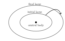
\end{aligned} ψ 0 ( x ( t 0 ) ) ψ f ( x ( t f ) ) = 0 , = 0 . For example, an orbital-transfer problem may require a spacecraft to begin somewhere on one orbit and end somewhere on another orbit without prescribing the exact position on either orbit.
Figure 2: A locus-to-locus transfer constrains endpoints to lie on sets rather than at prescribed points.
This broader boundary formulation substantially enlarges the class of problems that can be modeled.
The dynamics and boundary conditions may admit many feasible controls. Therefore, feasibility alone does not identify a unique preferred solution.
A performance index assigns a scalar measure to each admissible process:
J = Φ ( x ( t 0 ) , t 0 , x ( t f ) , t f , q ) + ∫ t 0 t f L ( x ( t ) , u ( t ) , t , q ) d t . J
=
\Phi
\bigl(
\boldsymbol{x}(t_0),
t_0,
\boldsymbol{x}(t_f),
t_f,
\boldsymbol{q}
\bigr)
+
\int_{t_0}^{t_f}
L
\bigl(
\boldsymbol{x}(t),
\boldsymbol{u}(t),
t,
\boldsymbol{q}
\bigr)
\,\mathrm{d} t. J = Φ ( x ( t 0 ) , t 0 , x ( t f ) , t f , q ) + ∫ t 0 t f L ( x ( t ) , u ( t ) , t , q ) d t . The endpoint term Φ \Phi Φ Mayer term . The integral term is called the Lagrange term . Their combination is commonly called the Bolza form .
A pure endpoint cost has the form
J = Φ ( x ( t 0 ) , t 0 , x ( t f ) , t f , q ) . J
=
\Phi
\bigl(
\boldsymbol{x}(t_0),
t_0,
\boldsymbol{x}(t_f),
t_f,
\boldsymbol{q}
\bigr). J = Φ ( x ( t 0 ) , t 0 , x ( t f ) , t f , q ) . A pure running cost has the form
J = ∫ t 0 t f L ( x , u , t , q ) d t . J
=
\int_{t_0}^{t_f}
L(\boldsymbol{x},\boldsymbol{u},t,\boldsymbol{q})\,\mathrm{d} t. J = ∫ t 0 t f L ( x , u , t , q ) d t . The general combination is
J = Φ + ∫ t 0 t f L d t . J
=
\Phi
+
\int_{t_0}^{t_f}L\,\mathrm{d} t. J = Φ + ∫ t 0 t f L d t . Fuel-Optimal Interpretation ¶ Suppose spacecraft mass satisfies
m ˙ ( t ) = − T ( t ) I s p g 0 , \dot{m}(t)
=
-
\frac{T(t)}{I_{\mathrm{sp}}g_0}, m ˙ ( t ) = − I sp g 0 T ( t ) , where T ( t ) T(t) T ( t ) I s p I_{\mathrm{sp}} I sp g 0 g_0 g 0
Integrating,
m ( t ) = m ( t 0 ) − ∫ t 0 t T ( τ ) I s p g 0 d τ . m(t)
=
m(t_0)
-
\int_{t_0}^{t}
\frac{T(\tau)}
{I_{\mathrm{sp}}g_0}
\,\mathrm{d}\tau. m ( t ) = m ( t 0 ) − ∫ t 0 t I sp g 0 T ( τ ) d τ . Minimizing fuel consumption is equivalent to maximizing final mass:
max m ( t f ) . \max m(t_f). max m ( t f ) . This can be written as a minimization:
min [ − m ( t f ) ] . \min\left[-m(t_f)\right]. min [ − m ( t f ) ] . More generally,
max F ⟺ min ( − F ) . \max F
\quad\Longleftrightarrow\quad
\min(-F). max F ⟺ min ( − F ) . The General Optimal Control Problem ¶ A standard optimal control problem is:
min u ( ⋅ ) , q , t 0 , t f J \min_{\boldsymbol{u}(\cdot),\,\boldsymbol{q},\,t_0,\,t_f}
J u ( ⋅ ) , q , t 0 , t f min J with
J = Φ ( x ( t 0 ) , t 0 , x ( t f ) , t f , q ) + ∫ t 0 t f L ( x ( t ) , u ( t ) , t , q ) d t , J
=
\Phi
\bigl(
\boldsymbol{x}(t_0),
t_0,
\boldsymbol{x}(t_f),
t_f,
\boldsymbol{q}
\bigr)
+
\int_{t_0}^{t_f}
L
\bigl(
\boldsymbol{x}(t),
\boldsymbol{u}(t),
t,
\boldsymbol{q}
\bigr)\,\mathrm{d} t, J = Φ ( x ( t 0 ) , t 0 , x ( t f ) , t f , q ) + ∫ t 0 t f L ( x ( t ) , u ( t ) , t , q ) d t , subject to
x ˙ = f ( x , u , t , q ) , \dot{\boldsymbol{x}}
=
\boldsymbol{f}(\boldsymbol{x},\boldsymbol{u},t,\boldsymbol{q}), x ˙ = f ( x , u , t , q ) , and
ϕ ( x ( t 0 ) , t 0 , x ( t f ) , t f , q ) = 0 . \boldsymbol{\phi}
\bigl(
\boldsymbol{x}(t_0),
t_0,
\boldsymbol{x}(t_f),
t_f,
\boldsymbol{q}
\bigr)
=
\boldsymbol{0}. ϕ ( x ( t 0 ) , t 0 , x ( t f ) , t f , q ) = 0 . Additional path constraints may also be imposed:
g ( x ( t ) , u ( t ) , t , q ) ≤ 0 . \boldsymbol{g}
\bigl(
\boldsymbol{x}(t),
\boldsymbol{u}(t),
t,
\boldsymbol{q}
\bigr)
\le
\boldsymbol{0}. g ( x ( t ) , u ( t ) , t , q ) ≤ 0 . Why Arbitrary Control Search Is Inadequate ¶ One might attempt to choose candidate controls, integrate the dynamics, evaluate the cost, and retain the best result. This approach is generally ineffective because:
the control is an infinite-dimensional function;
most arbitrary controls may violate boundary conditions;
the number of admissible alternatives is uncountably infinite;
random search provides no guarantee of stationarity or optimality.
A systematic variational framework is therefore needed. The next step is to convert the constrained optimal control problem into an augmented calculus-of-variations problem and derive its first-order necessary conditions.
Chapter Summary ¶ The key results are:
A free endpoint parameter produces an additional transversality or natural boundary condition.
For fixed terminal state and free final time,
[ L − x ˙ L x ˙ ] t f = 0. \left[
L-\dot{x}L_{\dot{x}}
\right]_{t_f}
=
0. [ L − x ˙ L x ˙ ] t f = 0. For fixed final time and free terminal state,
L x ˙ ( t f ) = 0. L_{\dot{x}}(t_f)=0. L x ˙ ( t f ) = 0. Boundary terms must be interpreted as products involving endpoint variations. One must determine from the problem statement which factor is constrained to vanish.
The Euler–Lagrange equation governs the interior path, while natural and transversality conditions govern the endpoints.
Gradients, Hessians, and Jacobians provide the derivative notation required for vector-valued optimal control problems.
A general dynamical system can be written as
x ˙ = f ( x , u , t , q ) . \dot{\boldsymbol{x}}
=
\boldsymbol{f}(\boldsymbol{x},\boldsymbol{u},t,\boldsymbol{q}). x ˙ = f ( x , u , t , q ) . General boundary conditions are expressed as
ϕ ( x ( t 0 ) , t 0 , x ( t f ) , t f , q ) = 0 . \boldsymbol{\phi}
\bigl(
\boldsymbol{x}(t_0),
t_0,
\boldsymbol{x}(t_f),
t_f,
\boldsymbol{q}
\bigr)
=
\boldsymbol{0}. ϕ ( x ( t 0 ) , t 0 , x ( t f ) , t f , q ) = 0 . The general Bolza performance index is
J = Φ + ∫ t 0 t f L d t . J
=
\Phi
+
\int_{t_0}^{t_f}L\,\mathrm{d} t. J = Φ + ∫ t 0 t f L d t . Dynamics and boundary conditions determine feasibility; the performance index determines preference among feasible processes.