From Optimization to Optimal Control

Optimal control is concerned with choosing the best possible evolution of a dynamical system. The word best must always be interpreted relative to a clearly defined performance measure. Depending on the application, one may wish to minimize travel time, energy consumption, fuel use, tracking error, vibration, or economic cost. In other applications, the objective may be to maximize profit, harvested energy, range, or reliability.

The central ideas of optimal control are easiest to understand by first returning to ordinary scalar optimization. In scalar optimization, the unknown is a number. In optimal control, the unknown is an entire function of time. The mathematical transition from optimizing a number to optimizing a function is the key conceptual step developed in this section.

Optimization as Efficient Decision Making¶

Optimization appears whenever a task can be accomplished in more than one way and some alternatives are preferred over others. Everyday scheduling, route planning, engineering design, and resource allocation all possess the same basic structure:

there is a decision to be made;
there is a goal or objective;
there are constraints that restrict what is possible;
there may be many feasible alternatives;
one seeks the alternative that performs best according to a chosen metric.

For example, suppose a person must complete grocery shopping. The task can be completed by many different routes through the store. One route may minimize time, while another may minimize walking distance or physical effort. The optimal route therefore depends on the chosen objective.

The Elements of an Optimization Problem¶

A generic finite-dimensional optimization problem can be written as

\min_{\boldsymbol{x}\in\mathbb{R}^n} f(\boldsymbol{x})

(1)

subject to

\begin{aligned} g_i(\boldsymbol{x}) &\le 0, \qquad i=1,\ldots,m,\\ h_j(\boldsymbol{x}) &=0, \qquad j=1,\ldots,p. \end{aligned}

(2)

Here:

$\boldsymbol{x}\in\mathbb{R}^n$ is the vector of decision variables;
$f:\mathbb{R}^n\rightarrow\mathbb{R}$ is the objective function;
$g_i$ are inequality constraints;
$h_j$ are equality constraints.

The set of all points satisfying the constraints is called the feasible set:

\mathcal{F} = \left\{ \boldsymbol{x}\in\mathbb{R}^n: g_i(\boldsymbol{x})\le 0,\; h_j(\boldsymbol{x})=0 \right\}.

(3)

The grocery-shopping example illustrates infeasibility. If the complete task must be finished in two minutes, no physically realizable route may satisfy the time constraint. If the allowed time is increased to three hours, the feasible set may become nonempty.

The Objective Function and the Meaning of “Optimal”¶

The objective function is the numerical quantity used to compare feasible solutions. For a minimization problem, a feasible point $\boldsymbol{x}^{*}$ is globally optimal if

f(\boldsymbol{x}^{*})\le f(\boldsymbol{x}) \qquad \forall \boldsymbol{x}\in\mathcal{F}.

(5)

For a maximization problem, $\boldsymbol{x}^{*}$ is globally optimal if

f(\boldsymbol{x}^{*})\ge f(\boldsymbol{x}) \qquad \forall \boldsymbol{x}\in\mathcal{F}.

(6)

Different objective functions generally produce different optimal solutions. For the same physical task, minimizing elapsed time may lead to a different decision than minimizing energy expenditure.

Scalar Functions¶

The simplest optimization setting is a scalar-valued function of a scalar variable:

f:\mathbb{R}\rightarrow\mathbb{R}, \qquad y=f(x).

(11)

The input $x$ is a real number, and the output $f(x)$ is also a real number. For a smooth function, classical calculus provides useful necessary and sufficient conditions for identifying local minima and maxima.

Critical Points and the First-Derivative Condition¶

Suppose $f$ is differentiable. At an interior local minimum or maximum, the slope must vanish under standard regularity assumptions:

\frac{df}{dx}(x^*)=0.

(12)

For the smooth functions considered here, critical points are obtained by solving

f'(x)=0.

(14)

Let

x_1,x_2,\ldots,x_N

(15)

denote all roots of this equation. These points are only candidates for extrema. A zero derivative does not by itself prove that a point is a minimum or maximum.

Why the first derivative vanishes¶

If $x^*$ is an interior local minimum and $f$ is differentiable, then for sufficiently small $h$ ,

f(x^*+h)\ge f(x^*).

(16)

For $h>0$ ,

\frac{f(x^*+h)-f(x^*)}{h}\ge 0,

(17)

while for $h<0$ ,

\frac{f(x^*+h)-f(x^*)}{h}\le 0.

(18)

Taking the limit $h\rightarrow 0$ from the right and left implies

f'(x^*)=0.

(19)

This result is a necessary condition for a smooth interior optimum, but it is not sufficient.

The Second-Derivative Test¶

The second derivative describes local curvature.

The interpretation follows from a second-order Taylor expansion:

f(x_c+h) = f(x_c) + f'(x_c)h + \frac{1}{2}f''(x_c)h^2 + o(h^2).

(23)

Because $f'(x_c)=0$ ,

f(x_c+h)-f(x_c) = \frac{1}{2}f''(x_c)h^2 + o(h^2).

(24)

Since $h^2\ge 0$ , the sign of $f''(x_c)$ determines whether nearby function values are larger or smaller.

Stationary Points That Are Not Extrema¶

A stationary point need not be a minimum or maximum.

Consider

f(x)=x^3.

(25)

Then

f'(x)=3x^2,

(26)

f'(0)=0.

(27)

However, $x=0$ is neither a local minimum nor a local maximum, because $f(x)<0$ for $x<0$ and $f(x)>0$ for $x>0$ .

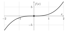
A stationary inflection point: f'(0)=0, but x=0 is neither a local minimum nor a local maximum. — Figure 1:A stationary inflection point: $f'(0)=0$ , but $x=0$ is neither a local minimum nor a local maximum.

Local and Global Extrema¶

A local optimum is best only in a neighborhood. A global optimum is best over the entire admissible domain.

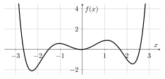
Figure 2:A smooth function may have several local extrema. Only one may be globally optimal.

For a smooth function with finitely many local maxima $x_1,\ldots,x_k$ , the global maximum among those candidates is found by comparing their objective values:

x^* = \operatorname*{arg\,max}_{x_i,\;i=1,\ldots,k} f(x_i).

(31)

Constrained Scalar Optimization¶

Now consider

\max_{x\in[a,b]} f(x).

(32)

The feasible set is the closed interval

\mathcal{F}=[a,b].

(33)

A crucial point is that the optimizer may lie at a boundary:

x^*=a \qquad\text{or}\qquad x^*=b.

(34)

At a boundary optimum, the derivative need not be zero.

Why the derivative test can fail¶

Consider

f(x)=x, \qquad x\in[0,1].

(35)

Then

f'(x)=1

(36)

for every $x\in[0,1]$ . There is no solution of $f'(x)=0$ , yet the maximum is clearly

x^*=1, \qquad f(x^*)=1.

(37)

Thus, the equation

f'(x)=0

(38)

detects only smooth interior stationary points. It does not detect active-boundary optima.

A Systematic Procedure on a Closed Interval¶

If $f$ is continuous on $[a,b]$ , the extreme value theorem guarantees that $f$ attains both a global minimum and a global maximum on $[a,b]$ .

A systematic procedure is:

solve

f'(x)=0

(39)

for all critical points in $(a,b)$ ;

evaluate $f$ at every interior critical point;
evaluate the endpoints:

f(a),\qquad f(b);

(40)

compare all candidate values.

Therefore,

\max_{x\in[a,b]} f(x) = \max \left\{ f(a), f(b), f(x_1), \ldots, f(x_N) \right\},

(41)

where $x_1,\ldots,x_N$ are the critical points in $(a,b)$ .

One-Sided Neighborhoods at a Boundary¶

At an interior local maximum $x^*$ , one compares $f(x^*)$ to function values on both sides. At a right boundary $b$ , only feasible perturbations to the left are allowed.

Thus, $b$ is a local maximum relative to the feasible set $[a,b]$ if there exists $\delta>0$ such that

f(b)\ge f(x), \qquad x\in[b-\delta,b].

(48)

Similarly, $a$ is a local maximum relative to $[a,b]$ if there exists $\delta>0$ such that

f(a)\ge f(x), \qquad x\in[a,a+\delta].

(49)

These are one-sided optimality statements because the feasible set restricts allowable perturbations.

Maximum Value Versus Maximizing Argument¶

There is an important distinction between the value of the objective and the point at which that value occurs.

The maximum value is

\max_{x\in[a,b]} f(x).

(50)

The maximizing argument is

x^* = \operatorname*{arg\,max}_{x\in[a,b]} f(x).

(51)

The first expression returns a number in the range of $f$ . The second returns a point in the domain of $f$ .

For example, if

f(x)=-(x-2)^2+5,

(52)

then

\max_{x\in\mathbb{R}} f(x)=5,

(53)

whereas

\operatorname*{arg\,max}_{x\in\mathbb{R}} f(x)=2.

(54)

If several points yield the same maximum value, the argmax is a set:

\operatorname*{arg\,max}_{x\in\mathcal{F}} f(x) = \left\{ x\in\mathcal{F}: f(x)=\max_{z\in\mathcal{F}} f(z) \right\}.

(55)

A Maximum-Principle Viewpoint¶

A derivative-free statement of optimality is

f(x^*)\ge f(x) \qquad \forall x\in\mathcal{F}.

(56)

Equivalently,

x^*\in\operatorname*{arg\,max}_{x\in\mathcal{F}} f(x).

(57)

This statement is more general than the condition $f'(x^*)=0$ because it remains meaningful when:

the optimum lies on the boundary;
the function is nonsmooth;
the decision variable is multidimensional;
the feasible set is discrete;
derivatives do not exist or are difficult to compute.

Derivative conditions are powerful computational tools when their assumptions hold, but they are not the definition of optimality.

From Points to Functions¶

Classical scalar optimization searches for a number:

x^*\in\mathbb{R}.

(58)

Optimal control searches for one or more functions of time:

\boldsymbol{u}^*(t), \qquad \boldsymbol{x}^*(t).

(59)

The unknown is therefore an entire trajectory, not a single point.

A standard optimal control problem has the form

\min_{\boldsymbol{u}(\cdot)} J[\boldsymbol{x}(\cdot),\boldsymbol{u}(\cdot)]

(60)

subject to the differential equation

\dot{\boldsymbol{x}}(t) = \boldsymbol{f}\bigl(\boldsymbol{x}(t),\boldsymbol{u}(t),t\bigr),

(61)

boundary conditions such as

\boldsymbol{x}(t_0)=\boldsymbol{x}_0,

(62)

and possibly path constraints

\boldsymbol{g}\bigl(\boldsymbol{x}(t),\boldsymbol{u}(t),t\bigr)\le \boldsymbol{0}.

(63)

Functions and Functionals¶

A function maps numbers or vectors to numbers or vectors. For example,

f:\mathbb{R}\rightarrow\mathbb{R}.

(64)

A functional maps an entire function to a number:

J:\mathcal{U}\rightarrow\mathbb{R},

(65)

where $\mathcal{U}$ is a space of admissible functions.

A common functional is

J[u] = \int_{t_0}^{t_f} L\bigl(u(t),t\bigr)\,dt.

(66)

The input to $J$ is the complete function $u(t)$ , while the output is a scalar.

A Route-Planning Interpretation¶

Suppose a traveler wishes to move from an initial location to a destination. A route can be represented by a path

\boldsymbol{r}(t) = \begin{bmatrix} x(t)\\ y(t) \end{bmatrix}.

(68)

Many paths may connect the same endpoints:

\boldsymbol{r}(t_0)=\boldsymbol{r}_0, \qquad \boldsymbol{r}(t_f)=\boldsymbol{r}_f.

(69)

A minimum-time problem seeks

\boldsymbol{r}^*(\cdot) \in \operatorname*{arg\,min}_{\boldsymbol{r}(\cdot)} t_f,

(70)

subject to kinematic, road, and speed constraints.

A minimum-distance problem instead minimizes

J[\boldsymbol{r}] = \int_{t_0}^{t_f} \left\| \dot{\boldsymbol{r}}(t) \right\|\,dt.

(71)

The two formulations may produce different paths. Again, the meaning of optimality depends on the performance index.

The Conceptual Transition¶

The progression from elementary optimization to optimal control can be summarized as follows:

Concept	Static optimization	Optimal control
Unknown	Point $\boldsymbol{x}$	Function $\boldsymbol{u}(t)$ or trajectory $\boldsymbol{x}(t)$
Objective	$f(\boldsymbol{x})$	Functional $J[\boldsymbol{x},\boldsymbol{u}]$
Constraints	Algebraic	Differential and algebraic
Solution	Optimal point	Optimal path or control history
Mathematical tools	Calculus, nonlinear programming	Calculus of variations, maximum principle, dynamic programming, direct transcription

Chapter Summary¶

The main ideas are:

Optimization selects the best feasible decision according to a specified performance measure.
A problem may be infeasible if its constraints cannot be satisfied.
For a smooth scalar function, interior critical points satisfy

f'(x)=0.

(72)

The second derivative classifies nondegenerate critical points:

f''(x)>0 \Rightarrow \text{local minimum},

(73)

f''(x)<0 \Rightarrow \text{local maximum}.

(74)

A critical point need not be an extremum.
Local extrema are not necessarily global extrema.
In constrained optimization, the optimizer may occur on the boundary, where the derivative need not vanish.
The expression

\max_{x\in\mathcal{F}} f(x)

(75)

gives the optimal value, while

\operatorname*{arg\,max}_{x\in\mathcal{F}} f(x)

(76)

gives the maximizing argument.

Optimal control extends optimization from points to functions.
A functional maps a function to a scalar.

Connection. Optimizing trajectories requires a space in which functions themselves can vary, so the scalar ideas above now give way to function spaces and functionals.