Function Spaces, Functionals, and the Calculus of Variations
Optimal control is fundamentally different from ordinary finite-dimensional optimization because the unknown is generally not a point. Instead, the unknown is an entire function of time. A control input
u ( t ) \boldsymbol{u}(t) u ( t ) assigns a command at every instant, while the corresponding state trajectory
x ( t ) \boldsymbol{x}(t) x ( t ) describes the evolution of the system over an interval of time.
This distinction requires a new mathematical framework. Ordinary calculus studies changes in numbers or vectors. The calculus of variations studies changes in entire functions. The purpose of this section is to establish the foundational distinctions among points, functions, functionals, differences, and variations, and then derive the first-order necessary condition for the classical fixed-endpoint problem in the calculus of variations.
The final result is the Euler–Lagrange equation:
∂ L ∂ x − d d t ( ∂ L ∂ x ˙ ) = 0. \frac{\partial L}{\partial x}
-
\frac{\,\mathrm{d}}{\,\mathrm{d} t}
\left(
\frac{\partial L}{\partial \dot{x}}
\right)
=0. ∂ x ∂ L − d t d ( ∂ x ˙ ∂ L ) = 0. Points and Functions ¶ Points in finite-dimensional space ¶ A point in n n n
x ∈ R n . \boldsymbol{x}\in\mathbb{R}^n. x ∈ R n . In component form,
x = [ x 1 x 2 ⋮ x n ] . \boldsymbol{x}
=
\begin{bmatrix}
x_1\\
x_2\\
\vdots\\
x_n
\end{bmatrix}. x = ⎣ ⎡ x 1 x 2 ⋮ x n ⎦ ⎤ . The object x \boldsymbol{x} x n n n
Vector-valued functions ¶ A vector-valued function of time is written as
x ( ⋅ ) ∈ Ω , \boldsymbol{x}(\cdot)\in\Omega, x ( ⋅ ) ∈ Ω , where Ω \Omega Ω t t t
x ( t ) = [ x 1 ( t ) x 2 ( t ) ⋮ x n ( t ) ] ∈ R n . \boldsymbol{x}(t)
=
\begin{bmatrix}
x_1(t)\\
x_2(t)\\
\vdots\\
x_n(t)
\end{bmatrix}
\in\mathbb{R}^n. x ( t ) = ⎣ ⎡ x 1 ( t ) x 2 ( t ) ⋮ x n ( t ) ⎦ ⎤ ∈ R n . The function x ( ⋅ ) \boldsymbol{x}(\cdot) x ( ⋅ ) R n \mathbb{R}^n R n t t t x ( t ) \boldsymbol{x}(t) x ( t ) R n \mathbb{R}^n R n
A function space may include smoothness, continuity, endpoint, or integrability requirements. Examples include
C ( [ t 0 , t f ] ) = { x : [ t 0 , t f ] → R | x is continuous } , C 1 ( [ t 0 , t f ] ) = { x : [ t 0 , t f ] → R | x and x ˙ are continuous } . \begin{aligned}
C([t_0,t_f]) &=
\left\{
x:[t_0,t_f]\rightarrow\mathbb{R}
\; \middle| \;
x \text{ is continuous}
\right\},\\
C^1([t_0,t_f]) &=
\left\{
x:[t_0,t_f]\rightarrow\mathbb{R}
\; \middle| \;
x \text{ and }\dot{x}
\text{ are continuous}
\right\}.
\end{aligned} C ([ t 0 , t f ]) C 1 ([ t 0 , t f ]) = { x : [ t 0 , t f ] → R ∣ x is continuous } , = { x : [ t 0 , t f ] → R ∣ x and x ˙ are continuous } . Functions and Functionals ¶ Ordinary functions ¶ An ordinary function maps points to points. For example,
f : R n → R m . \boldsymbol{f}:\mathbb{R}^n\rightarrow\mathbb{R}^m. f : R n → R m . Given an input x ∈ R n \boldsymbol{x}\in\mathbb{R}^n x ∈ R n
f ( x ) ∈ R m . \boldsymbol{f}(\boldsymbol{x})\in\mathbb{R}^m. f ( x ) ∈ R m . In the scalar case,
f : R n → R . f:\mathbb{R}^n\rightarrow\mathbb{R}. f : R n → R . Functionals ¶ A functional maps an entire function to a scalar:
J : Ω → R . J:\Omega\rightarrow\mathbb{R}. J : Ω → R . Thus,
x ( ⋅ ) ∈ Ω ⟹ J [ x ] ∈ R . x(\cdot)\in\Omega
\quad\Longrightarrow\quad
J[x]\in\mathbb{R}. x ( ⋅ ) ∈ Ω ⟹ J [ x ] ∈ R . A fundamental example is the integral functional
J [ x ] = ∫ a b x ( τ ) d τ . J[x]
=
\int_a^b x(\tau)\,\mathrm{d}\tau. J [ x ] = ∫ a b x ( τ ) d τ . The variable τ \tau τ
Why the Integration Variable Is Not an Output Variable ¶ Consider
J [ x ] = ∫ t 0 t f L ( x ( t ) , x ˙ ( t ) , t ) d t . J[x]
=
\int_{t_0}^{t_f}
L\bigl(x(t),\dot{x}(t),t\bigr)\,\mathrm{d} t. J [ x ] = ∫ t 0 t f L ( x ( t ) , x ˙ ( t ) , t ) d t . Although the integrand depends explicitly on t t t J J J t t t [ t 0 , t f ] [t_0,t_f] [ t 0 , t f ]
The result depends on the chosen function x ( ⋅ ) x(\cdot) x ( ⋅ ) L L L
Control as a Function ¶ A control input is usually a function of time:
u : [ t 0 , t f ] → R m . \boldsymbol{u}:[t_0,t_f]\rightarrow\mathbb{R}^m. u : [ t 0 , t f ] → R m . At each time t t t
u ( t ) ∈ R m . \boldsymbol{u}(t)\in\mathbb{R}^m. u ( t ) ∈ R m . For a vehicle, controls might include steering angle, throttle, and braking force. The defining feature of a control is that it can be selected, subject to allowable limits such as
u min ≤ u ( t ) ≤ u max . \boldsymbol{u}_{\min}
\le
\boldsymbol{u}(t)
\le
\boldsymbol{u}_{\max}. u m i n ≤ u ( t ) ≤ u m a x . The goal of optimal control is to determine an entire admissible function u ∗ ( t ) \boldsymbol{u}^*(t) u ∗ ( t )
Differences and Variations ¶ Difference between points ¶ Let
x ∈ R n \boldsymbol{x}\in\mathbb{R}^n x ∈ R n and consider a second point
y = x + Δ x . \boldsymbol{y}
=
\boldsymbol{x}
+
\Delta\boldsymbol{x}. y = x + Δ x . Then
Δ x = y − x \Delta\boldsymbol{x}
=
\boldsymbol{y}
-
\boldsymbol{x} Δ x = y − x is the difference or increment between two points.
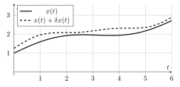
Variation of a function ¶ For a function x ( ⋅ ) x(\cdot) x ( ⋅ )
x ~ ( t ) = x ( t ) + δ x ( t ) . \widetilde{x}(t)
=
x(t)
+
\delta x(t). x ( t ) = x ( t ) + δ x ( t ) . Here δ x ( t ) \delta x(t) δ x ( t ) x ( t ) x(t) x ( t )
Figure 1: A variation perturbs the entire function, not merely one point.
Increments of Functions and Functionals ¶ Increment of an ordinary function ¶ Let
f : R n → R . f:\mathbb{R}^n\rightarrow\mathbb{R}. f : R n → R . The increment in f f f Δ q \Delta\boldsymbol{q} Δ q
Δ f = f ( q + Δ q ) − f ( q ) . \Delta f
=
f(\boldsymbol{q}+\Delta\boldsymbol{q})
-
f(\boldsymbol{q}). Δ f = f ( q + Δ q ) − f ( q ) . A first-order Taylor expansion gives
Δ f = ∇ f ( q ) ⊤ Δ q + O ( ∥ Δ q ∥ 2 ) . \Delta f
=
\nabla f(\boldsymbol{q})^\top\Delta\boldsymbol{q}
+
\mathcal{O}\left(\|\Delta\boldsymbol{q}\|^2\right). Δ f = ∇ f ( q ) ⊤ Δ q + O ( ∥Δ q ∥ 2 ) . Increment of a functional ¶ Let
J : Ω → R . J:\Omega\rightarrow\mathbb{R}. J : Ω → R . The increment of J J J
q ( ⋅ ) + δ q ( ⋅ ) q(\cdot)+\delta q(\cdot) q ( ⋅ ) + δ q ( ⋅ ) is
Δ J = J [ q + δ q ] − J [ q ] . \Delta J
=
J[q+\delta q]
-
J[q]. Δ J = J [ q + δ q ] − J [ q ] . The first-order portion of this increment is called the first variation:
Formally,
J [ q + ϵ η ] = J [ q ] + ϵ δ J [ q ; η ] + O ( ϵ 2 ) , J[q+\epsilon\eta]
=
J[q]
+
\epsilon\,\delta J[q;\eta]
+
\mathcal{O}(\epsilon^2), J [ q + ϵη ] = J [ q ] + ϵ δ J [ q ; η ] + O ( ϵ 2 ) , where η ( t ) \eta(t) η ( t ) ϵ \epsilon ϵ
Equivalently,
δ J [ q ; η ] = d d ϵ J [ q + ϵ η ] ∣ ϵ = 0 . \delta J[q;\eta]
=
\left.
\frac{\,\mathrm{d}}{\,\mathrm{d}\epsilon}
J[q+\epsilon\eta]
\right|_{\epsilon=0}. δ J [ q ; η ] = d ϵ d J [ q + ϵη ] ∣ ∣ ϵ = 0 . Local and Global Minima ¶ Minima of ordinary functions ¶ A point q ∗ ∈ R n \boldsymbol{q}^*\in\mathbb{R}^n q ∗ ∈ R n f f f q ∗ \boldsymbol{q}^* q ∗
f ( q ∗ + Δ q ) ≥ f ( q ∗ ) f(\boldsymbol{q}^*+\Delta\boldsymbol{q})
\ge
f(\boldsymbol{q}^*) f ( q ∗ + Δ q ) ≥ f ( q ∗ ) for all sufficiently small Δ q \Delta\boldsymbol{q} Δ q
It is a global minimum if
f ( q ) ≥ f ( q ∗ ) ∀ q ∈ R n . f(\boldsymbol{q})
\ge
f(\boldsymbol{q}^*)
\qquad
\forall \boldsymbol{q}\in\mathbb{R}^n. f ( q ) ≥ f ( q ∗ ) ∀ q ∈ R n . Extrema of functionals ¶ A function x ∗ ( ⋅ ) ∈ Ω x^*(\cdot)\in\Omega x ∗ ( ⋅ ) ∈ Ω J J J
J [ x ∗ + δ x ] ≥ J [ x ∗ ] J[x^*+\delta x]
\ge
J[x^*] J [ x ∗ + δ x ] ≥ J [ x ∗ ] for all sufficiently small admissible variations δ x ( ⋅ ) \delta x(\cdot) δ x ( ⋅ )
It is a global minimum if
J [ x ] ≥ J [ x ∗ ] ∀ x ( ⋅ ) ∈ Ω . J[x]
\ge
J[x^*]
\qquad
\forall x(\cdot)\in\Omega. J [ x ] ≥ J [ x ∗ ] ∀ x ( ⋅ ) ∈ Ω. More generally, minima and maxima of functionals are referred to as extrema.
Ordinary Calculus and the Calculus of Variations ¶ Ordinary calculus determines extrema of functions by analyzing derivatives with respect to finite-dimensional variables.
For example, if
f : R → R , f:\mathbb{R}\rightarrow\mathbb{R}, f : R → R , then an interior extremum satisfies
d f d x = 0. \frac{\,\mathrm{d} f}{\,\mathrm{d} x}=0. d x d f = 0. The calculus of variations performs an analogous task for functionals. An extremizing function x ∗ ( ⋅ ) x^*(\cdot) x ∗ ( ⋅ )
for all admissible first-order variations.
The Classical Fixed-Endpoint Problem ¶ Consider the functional
J [ x ] = ∫ t 0 t f L ( x ( t ) , x ˙ ( t ) , t ) d t , J[x]
=
\int_{t_0}^{t_f}
L\bigl(x(t),\dot{x}(t),t\bigr)\,\mathrm{d} t, J [ x ] = ∫ t 0 t f L ( x ( t ) , x ˙ ( t ) , t ) d t , where L L L x ( t ) x(t) x ( t )
Assume that
x ( t 0 ) = x 0 , x ( t f ) = x f , \begin{aligned}
x(t_0)&=x_0,\\
x(t_f)&=x_f,
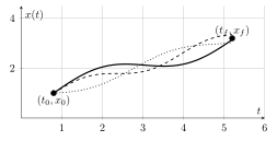
\end{aligned} x ( t 0 ) x ( t f ) = x 0 , = x f , and that t 0 t_0 t 0 t f t_f t f x 0 x_0 x 0 x f x_f x f
The objective is to determine a function
that makes J [ x ] J[x] J [ x ]
Figure 2: Many admissible functions can connect the same fixed endpoints. The calculus of variations identifies the extremizing path.
Admissible Variations ¶ Let the perturbed path be
x ~ ( t ) = x ( t ) + ϵ η ( t ) , \widetilde{x}(t)
=
x(t)
+
\epsilon\eta(t), x ( t ) = x ( t ) + ϵη ( t ) , where η ( t ) \eta(t) η ( t )
Because the endpoint values are fixed, the perturbed path must satisfy
x ~ ( t 0 ) = x 0 , x ~ ( t f ) = x f . \begin{aligned}
\widetilde{x}(t_0)&=x_0,\\
\widetilde{x}(t_f)&=x_f.
\end{aligned} x ( t 0 ) x ( t f ) = x 0 , = x f . Substituting (49)
x ( t 0 ) + ϵ η ( t 0 ) = x 0 , x ( t f ) + ϵ η ( t f ) = x f . \begin{aligned}
x(t_0)+\epsilon\eta(t_0)&=x_0,\\
x(t_f)+\epsilon\eta(t_f)&=x_f.
\end{aligned} x ( t 0 ) + ϵη ( t 0 ) x ( t f ) + ϵη ( t f ) = x 0 , = x f . Since x ( t 0 ) = x 0 x(t_0)=x_0 x ( t 0 ) = x 0 x ( t f ) = x f x(t_f)=x_f x ( t f ) = x f
η ( t 0 ) = 0 , η ( t f ) = 0. \eta(t_0)=0,
\qquad
\eta(t_f)=0. η ( t 0 ) = 0 , η ( t f ) = 0. Equivalently,
δ x ( t 0 ) = 0 , δ x ( t f ) = 0. \delta x(t_0)=0,
\qquad
\delta x(t_f)=0. δ x ( t 0 ) = 0 , δ x ( t f ) = 0. Derivation of the First Variation ¶ The first variation of (46)
δ J = δ ∫ t 0 t f L ( x , x ˙ , t ) d t . \delta J
=
\delta
\int_{t_0}^{t_f}
L\bigl(x,\dot{x},t\bigr)\,\mathrm{d} t. δ J = δ ∫ t 0 t f L ( x , x ˙ , t ) d t . Because the integration limits are fixed, the variation can be moved inside the integral:
δ J = ∫ t 0 t f δ L d t . \delta J
=
\int_{t_0}^{t_f}
\delta L\,\mathrm{d} t. δ J = ∫ t 0 t f δ L d t . To first order,
δ L = ∂ L ∂ x δ x + ∂ L ∂ x ˙ δ x ˙ . \delta L
=
\frac{\partial L}{\partial x}\delta x
+
\frac{\partial L}{\partial\dot{x}}
\delta\dot{x}. δ L = ∂ x ∂ L δ x + ∂ x ˙ ∂ L δ x ˙ . There is no term involving a variation δ t \delta t δ t t t t
Substitution into (55)
δ J = ∫ t 0 t f [ ∂ L ∂ x δ x + ∂ L ∂ x ˙ δ x ˙ ] d t . \delta J
=
\int_{t_0}^{t_f}
\left[
\frac{\partial L}{\partial x}\delta x
+
\frac{\partial L}{\partial\dot{x}}
\delta\dot{x}
\right]\,\mathrm{d} t. δ J = ∫ t 0 t f [ ∂ x ∂ L δ x + ∂ x ˙ ∂ L δ x ˙ ] d t . Dependence of δ x ˙ \delta \dot{x} δ x ˙ δ x \delta x δ x ¶ The variations δ x \delta x δ x δ x ˙ \delta\dot{x} δ x ˙
x ˙ ( t ) = d x d t . \dot{x}(t)
=
\frac{\,\mathrm{d} x}{\,\mathrm{d} t}. x ˙ ( t ) = d t d x . Under standard smoothness assumptions, variation and differentiation commute:
δ x ˙ = d d t δ x . \delta\dot{x}
=
\frac{\,\mathrm{d}}{\,\mathrm{d} t}\delta x. δ x ˙ = d t d δ x . Therefore,
δ J = ∫ t 0 t f [ ∂ L ∂ x δ x + ∂ L ∂ x ˙ d d t ( δ x ) ] d t . \delta J
=
\int_{t_0}^{t_f}
\left[
\frac{\partial L}{\partial x}\delta x
+
\frac{\partial L}{\partial\dot{x}}
\frac{\,\mathrm{d}}{\,\mathrm{d} t}(\delta x)
\right]\,\mathrm{d} t. δ J = ∫ t 0 t f [ ∂ x ∂ L δ x + ∂ x ˙ ∂ L d t d ( δ x ) ] d t . Integration by Parts ¶ Recall the integration-by-parts identity
∫ a b u ( t ) v ˙ ( t ) d t = u ( t ) v ( t ) ∣ a b − ∫ a b u ˙ ( t ) v ( t ) d t . \int_a^b u(t)\dot{v}(t)\,\mathrm{d} t
=
\left.
u(t)v(t)
\right|_a^b
-
\int_a^b \dot{u}(t)v(t)\,\mathrm{d} t. ∫ a b u ( t ) v ˙ ( t ) d t = u ( t ) v ( t ) ∣ a b − ∫ a b u ˙ ( t ) v ( t ) d t . Choose
u ( t ) = ∂ L ∂ x ˙ , v ( t ) = δ x ( t ) . u(t)
=
\frac{\partial L}{\partial\dot{x}},
\qquad
v(t)
=
\delta x(t). u ( t ) = ∂ x ˙ ∂ L , v ( t ) = δ x ( t ) . Then
∫ t 0 t f ∂ L ∂ x ˙ d d t ( δ x ) d t = ∂ L ∂ x ˙ δ x ∣ t 0 t f − ∫ t 0 t f d d t ( ∂ L ∂ x ˙ ) δ x d t . \begin{aligned}
\int_{t_0}^{t_f}
\frac{\partial L}{\partial\dot{x}}
\frac{\,\mathrm{d}}{\,\mathrm{d} t}(\delta x)
\,\mathrm{d} t
&=
\left.
\frac{\partial L}{\partial\dot{x}}
\delta x
\right|_{t_0}^{t_f}
\nonumber\\
&\quad
-
\int_{t_0}^{t_f}
\frac{\,\mathrm{d}}{\,\mathrm{d} t}
\left(
\frac{\partial L}{\partial\dot{x}}
\right)
\delta x
\,\mathrm{d} t.
\end{aligned} ∫ t 0 t f ∂ x ˙ ∂ L d t d ( δ x ) d t = ∂ x ˙ ∂ L δ x ∣ ∣ t 0 t f − ∫ t 0 t f d t d ( ∂ x ˙ ∂ L ) δ x d t . Substitution into (60)
δ J = ∫ t 0 t f [ ∂ L ∂ x − d d t ( ∂ L ∂ x ˙ ) ] δ x d t + ∂ L ∂ x ˙ δ x ∣ t 0 t f . \begin{aligned}
\delta J
&=
\int_{t_0}^{t_f}
\left[
\frac{\partial L}{\partial x}
-
\frac{\,\mathrm{d}}{\,\mathrm{d} t}
\left(
\frac{\partial L}{\partial\dot{x}}
\right)
\right]
\delta x
\,\mathrm{d} t
\nonumber\\
&\quad
+
\left.
\frac{\partial L}{\partial\dot{x}}
\delta x
\right|_{t_0}^{t_f}.
\end{aligned} δ J = ∫ t 0 t f [ ∂ x ∂ L − d t d ( ∂ x ˙ ∂ L ) ] δ x d t + ∂ x ˙ ∂ L δ x ∣ ∣ t 0 t f . Because the endpoints are fixed,
δ x ( t 0 ) = 0 , δ x ( t f ) = 0. \delta x(t_0)=0,
\qquad
\delta x(t_f)=0. δ x ( t 0 ) = 0 , δ x ( t f ) = 0. Hence the boundary term vanishes:
∂ L ∂ x ˙ δ x ∣ t 0 t f = 0. \left.
\frac{\partial L}{\partial\dot{x}}
\delta x
\right|_{t_0}^{t_f}
=
0. ∂ x ˙ ∂ L δ x ∣ ∣ t 0 t f = 0. Thus,
δ J = ∫ t 0 t f [ ∂ L ∂ x − d d t ( ∂ L ∂ x ˙ ) ] δ x d t . \delta J
=
\int_{t_0}^{t_f}
\left[
\frac{\partial L}{\partial x}
-
\frac{\,\mathrm{d}}{\,\mathrm{d} t}
\left(
\frac{\partial L}{\partial\dot{x}}
\right)
\right]
\delta x
\,\mathrm{d} t. δ J = ∫ t 0 t f [ ∂ x ∂ L − d t d ( ∂ x ˙ ∂ L ) ] δ x d t . The Fundamental Lemma of the Calculus of Variations ¶ Suppose g ( t ) g(t) g ( t ) [ t 0 , t f ] [t_0,t_f] [ t 0 , t f ]
∫ t 0 t f g ( t ) η ( t ) d t = 0 \int_{t_0}^{t_f}
g(t)\eta(t)\,\mathrm{d} t
=
0 ∫ t 0 t f g ( t ) η ( t ) d t = 0 for every sufficiently smooth function η ( t ) \eta(t) η ( t )
η ( t 0 ) = η ( t f ) = 0. \eta(t_0)=\eta(t_f)=0. η ( t 0 ) = η ( t f ) = 0. Then
g ( t ) = 0 ∀ t ∈ [ t 0 , t f ] . g(t)=0
\qquad
\forall t\in[t_0,t_f]. g ( t ) = 0 ∀ t ∈ [ t 0 , t f ] . Applying the lemma to (67) δ x ( t ) \delta x(t) δ x ( t )
∂ L ∂ x − d d t ( ∂ L ∂ x ˙ ) = 0. \frac{\partial L}{\partial x}
-
\frac{\,\mathrm{d}}{\,\mathrm{d} t}
\left(
\frac{\partial L}{\partial\dot{x}}
\right)
=
0. ∂ x ∂ L − d t d ( ∂ x ˙ ∂ L ) = 0. Interpretation of the Euler–Lagrange Equation ¶ The Euler–Lagrange equation is not the extremizing function itself. It is a differential equation that the extremizing function must satisfy.
The solution procedure is therefore:
compute
∂ L ∂ x ; \frac{\partial L}{\partial x}; ∂ x ∂ L ; compute
∂ L ∂ x ˙ ; \frac{\partial L}{\partial\dot{x}}; ∂ x ˙ ∂ L ; differentiate the latter with respect to time:
d d t ( ∂ L ∂ x ˙ ) ; \frac{\,\mathrm{d}}{\,\mathrm{d} t}
\left(
\frac{\partial L}{\partial\dot{x}}
\right); d t d ( ∂ x ˙ ∂ L ) ; form the Euler–Lagrange differential equation;
solve the differential equation subject to the endpoint conditions.
Worked Example: Minimizing the Integral of Squared Slope ¶ Consider
J [ x ] = ∫ t 0 t f 1 2 x ˙ 2 ( t ) d t J[x]
=
\int_{t_0}^{t_f}
\frac{1}{2}\dot{x}^2(t)\,\mathrm{d} t J [ x ] = ∫ t 0 t f 2 1 x ˙ 2 ( t ) d t subject to
x ( t 0 ) = x 0 , x ( t f ) = x f . x(t_0)=x_0,
\qquad
x(t_f)=x_f. x ( t 0 ) = x 0 , x ( t f ) = x f . Here,
L ( x , x ˙ , t ) = 1 2 x ˙ 2 . L(x,\dot{x},t)
=
\frac{1}{2}\dot{x}^2. L ( x , x ˙ , t ) = 2 1 x ˙ 2 . Then
∂ L ∂ x = 0 , \frac{\partial L}{\partial x}=0, ∂ x ∂ L = 0 , and
∂ L ∂ x ˙ = x ˙ . \frac{\partial L}{\partial\dot{x}}
=
\dot{x}. ∂ x ˙ ∂ L = x ˙ . The Euler–Lagrange equation becomes
0 − d d t ( x ˙ ) = 0 , 0
-
\frac{\,\mathrm{d}}{\,\mathrm{d} t}(\dot{x})
=
0, 0 − d t d ( x ˙ ) = 0 , or
Integrating twice gives
x ( t ) = c 1 t + c 2 . x(t)=c_1t+c_2. x ( t ) = c 1 t + c 2 . Using the endpoint conditions,
x ∗ ( t ) = x 0 + x f − x 0 t f − t 0 ( t − t 0 ) . x^*(t)
=
x_0
+
\frac{x_f-x_0}{t_f-t_0}
(t-t_0). x ∗ ( t ) = x 0 + t f − t 0 x f − x 0 ( t − t 0 ) . Thus, the extremizing path is the straight line joining the two endpoints.
Worked Example: A Functional with a Trivial Minimizer ¶ Consider
J [ x ] = ∫ a b x 2 ( t ) d t . J[x]
=
\int_a^b x^2(t)\,\mathrm{d} t. J [ x ] = ∫ a b x 2 ( t ) d t . Because
x 2 ( t ) ≥ 0 x^2(t)\ge 0 x 2 ( t ) ≥ 0 for all t t t
The lower bound is achieved by
x ∗ ( t ) = 0 , x^*(t)=0, x ∗ ( t ) = 0 , which yields
J [ x ∗ ] = 0. J[x^*]=0. J [ x ∗ ] = 0. The Euler–Lagrange equation confirms this result. Here
so
∂ L ∂ x = 2 x , ∂ L ∂ x ˙ = 0. \frac{\partial L}{\partial x}=2x,
\qquad
\frac{\partial L}{\partial\dot{x}}=0. ∂ x ∂ L = 2 x , ∂ x ˙ ∂ L = 0. Therefore,
and hence
x ∗ ( t ) = 0. x^*(t)=0. x ∗ ( t ) = 0. Let
x ( t ) ∈ R n \boldsymbol{x}(t)\in\mathbb{R}^n x ( t ) ∈ R n and consider
J [ x ] = ∫ t 0 t f L ( x ( t ) , x ˙ ( t ) , t ) d t . J[\boldsymbol{x}]
=
\int_{t_0}^{t_f}
L\bigl(\boldsymbol{x}(t),\dot{\boldsymbol{x}}(t),t\bigr)\,\mathrm{d} t. J [ x ] = ∫ t 0 t f L ( x ( t ) , x ˙ ( t ) , t ) d t . The Euler–Lagrange equation becomes
∂ L ∂ x − d d t ( ∂ L ∂ x ˙ ) = 0 . \frac{\partial L}{\partial\boldsymbol{x}}
-
\frac{\,\mathrm{d}}{\,\mathrm{d} t}
\left(
\frac{\partial L}{\partial\dot{\boldsymbol{x}}}
\right)
=
\boldsymbol{0}. ∂ x ∂ L − d t d ( ∂ x ˙ ∂ L ) = 0 . Componentwise,
∂ L ∂ x i − d d t ( ∂ L ∂ x ˙ i ) = 0 , i = 1 , … , n . \frac{\partial L}{\partial x_i}
-
\frac{\,\mathrm{d}}{\,\mathrm{d} t}
\left(
\frac{\partial L}{\partial\dot{x}_i}
\right)
=
0,
\qquad
i=1,\ldots,n. ∂ x i ∂ L − d t d ( ∂ x ˙ i ∂ L ) = 0 , i = 1 , … , n . Connection to Lagrangian Mechanics ¶ In analytical mechanics, the Lagrangian is often defined as
L ( q , q ˙ , t ) = T ( q , q ˙ , t ) − V ( q , t ) , \mathcal{L}(\boldsymbol{q},\dot{\boldsymbol{q}},t)
=
T(\boldsymbol{q},\dot{\boldsymbol{q}},t)
-
V(\boldsymbol{q},t), L ( q , q ˙ , t ) = T ( q , q ˙ , t ) − V ( q , t ) , where T T T V V V
The action functional is
S [ q ] = ∫ t 0 t f L ( q , q ˙ , t ) d t . \mathcal{S}[\boldsymbol{q}]
=
\int_{t_0}^{t_f}
\mathcal{L}(\boldsymbol{q},\dot{\boldsymbol{q}},t)\,\mathrm{d} t. S [ q ] = ∫ t 0 t f L ( q , q ˙ , t ) d t . Hamilton’s principle states that the physically realized trajectory renders the action stationary:
δ S = 0. \delta\mathcal{S}=0. δ S = 0. The resulting Euler–Lagrange equations are
∂ L ∂ q i − d d t ( ∂ L ∂ q ˙ i ) = 0. \frac{\partial\mathcal{L}}{\partial q_i}
-
\frac{\,\mathrm{d}}{\,\mathrm{d} t}
\left(
\frac{\partial\mathcal{L}}{\partial\dot{q}_i}
\right)
=
0. ∂ q i ∂ L − d t d ( ∂ q ˙ i ∂ L ) = 0. Thus, the same mathematical structure that determines stationary functionals also generates the equations of motion in classical mechanics.
Principle of Stationary Action ¶ The phrase principle of least action is commonly used, but the more precise statement is that the physical path makes the action stationary. The path may correspond to a minimum, maximum, or saddle-type stationary value depending on the problem.
Therefore,
δ S = 0 \delta\mathcal{S}=0 δ S = 0 is the fundamental first-order condition.
Important Assumptions in the Derivation ¶ The derivation of (71)
the endpoint times t 0 t_0 t 0 t f t_f t f
the endpoint values x ( t 0 ) x(t_0) x ( t 0 ) x ( t f ) x(t_f) x ( t f )
the admissible functions are sufficiently smooth;
the integrand L ( x , x ˙ , t ) L(x,\dot{x},t) L ( x , x ˙ , t )
the variation and time differentiation commute;
only first-order variation terms are retained.
When endpoint values or endpoint times are free, additional boundary conditions arise. These are called natural boundary conditions or transversality conditions.
Chapter Summary ¶ The principal ideas developed in this section are:
A point x ∈ R n \boldsymbol{x}\in\mathbb{R}^n x ∈ R n x ( ⋅ ) ∈ Ω \boldsymbol{x}(\cdot)\in\Omega x ( ⋅ ) ∈ Ω
An ordinary function maps points to values:
f : R n → R m . f:\mathbb{R}^n\rightarrow\mathbb{R}^m. f : R n → R m . A functional maps functions to real numbers:
J : Ω → R . J:\Omega\rightarrow\mathbb{R}. J : Ω → R . A finite-dimensional increment is denoted by Δ x \Delta\boldsymbol{x} Δ x δ x ( t ) \delta x(t) δ x ( t )
The first variation δ J \delta J δ J
For the fixed-endpoint problem
J [ x ] = ∫ t 0 t f L ( x , x ˙ , t ) d t , J[x]
=
\int_{t_0}^{t_f}
L(x,\dot{x},t)\,\mathrm{d} t, J [ x ] = ∫ t 0 t f L ( x , x ˙ , t ) d t , the first-order stationarity condition is
Integration by parts converts the dependence on δ x ˙ \delta\dot{x} δ x ˙ δ x \delta x δ x
Fixed endpoints imply
δ x ( t 0 ) = δ x ( t f ) = 0. \delta x(t_0)=\delta x(t_f)=0. δ x ( t 0 ) = δ x ( t f ) = 0. The resulting Euler–Lagrange equation is
∂ L ∂ x − d d t ( ∂ L ∂ x ˙ ) = 0. \frac{\partial L}{\partial x}
-
\frac{\,\mathrm{d}}{\,\mathrm{d} t}
\left(
\frac{\partial L}{\partial\dot{x}}
\right)
=
0. ∂ x ∂ L − d t d ( ∂ x ˙ ∂ L ) = 0. The Euler–Lagrange equation is a necessary condition, not a guarantee of a minimum.
The same equation appears in classical mechanics through Hamilton’s principle of stationary action.
Connection. Once interior variations are understood, the next question is what changes when the endpoints are not fixed; endpoint variations provide that extension.