Endpoint Variations and Transversality Conditions

The classical fixed-endpoint problem in the calculus of variations assumes that the initial time, final time, initial state, and final state are all prescribed. Under those assumptions, the first variation leads to the Euler–Lagrange equation, and the endpoint terms vanish because the endpoint variations are zero.

Many practical problems are less restrictive. A system may be required to reach a specified terminal state without prescribing the arrival time. Alternatively, the final time may be fixed while the final state is free. More general problems may allow both endpoint time and endpoint state to vary subject to geometric or algebraic constraints.

These cases produce additional necessary conditions known as transversality conditions. This section develops the endpoint variation identities, derives the free-final-time condition, discusses the free-final-state condition, and illustrates the results through a mechanical example.

Review of the Basic Functional¶

Consider the functional

J[x] = \int_{t_0}^{t_f} L\bigl(x(t),\dot{x}(t),t\bigr)\,\mathrm{d} t.

(1)

The variable $t$ is a dummy variable of integration. Therefore, after integration, $J[x]$ is not a function of the dummy variable $t$ . Instead, the value of the functional depends on:

the entire function $x(\cdot)$ ;
the corresponding derivative $\dot{x}(\cdot)$ ;
the endpoint parameters $t_0$ and $t_f$ ;
the integrand $L$ .

If $t_f$ is free, then changing $t_f$ can change the numerical value of the functional. Consequently, the first variation must include a term involving $\delta t_f$ .

Fixed and Free Endpoint Data¶

For the most restrictive scalar problem, all endpoint data are fixed:

\begin{aligned} t_0 &= \text{fixed},\\ t_f &= \text{fixed},\\ x(t_0)&=x_0,\\ x(t_f)&=x_f. \end{aligned}

(2)

The admissible variations satisfy

\delta x(t_0)=0, \qquad \delta x(t_f)=0.

(3)

A first extension is the free-final-time problem:

\begin{aligned} t_0 &= \text{fixed},\\ x(t_0)&=x_0,\\ x(t_f)&=x_f,\\ t_f & \text{ is free}. \end{aligned}

(4)

Here, the terminal state value is prescribed, but the time at which that value is reached is unknown.

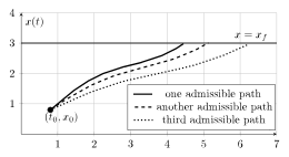
Geometric Interpretation of a Free Final Time¶

Suppose an admissible path begins at the fixed point

(t_0,x_0)

(5)

and must reach the prescribed terminal value $x_f$ . If $t_f$ is free, the endpoint may occur anywhere along the horizontal line

x=x_f.

(6)

When the terminal state is fixed but the terminal time is free, admissible trajectories may reach the line x=x_f at different times. — Figure 1:When the terminal state is fixed but the terminal time is free, admissible trajectories may reach the line $x=x_f$ at different times.

Variation of an Endpoint¶

The endpoint of a trajectory can change in two different ways:

the function itself may vary at the original endpoint time;
the endpoint time may move.

These effects must be distinguished carefully.

Let the nominal final endpoint be

\bigl(t_f,x_f\bigr), \qquad x_f=x(t_f).

(7)

After perturbation, let the endpoint become

\bigl(t_f+\delta t_f,\;x_f+\delta x_f\bigr).

(8)

The perturbed function is

\widetilde{x}(t) = x(t)+\delta x(t).

(9)

A first-order Taylor expansion gives

\begin{aligned} x_f+\delta x_f &= \widetilde{x}(t_f+\delta t_f) \nonumber\\ &= x(t_f+\delta t_f) + \delta x(t_f+\delta t_f) \nonumber\\ &\approx x(t_f) + \dot{x}(t_f)\delta t_f + \delta x(t_f). \end{aligned}

(10)

Since $x(t_f)=x_f$ , we obtain the endpoint variation identity

\boxed{ \delta x_f = \delta x(t_f) + \dot{x}(t_f)\delta t_f }.

(11)

Similarly, at the initial endpoint,

\boxed{ \delta x_0 = \delta x(t_0) + \dot{x}(t_0)\delta t_0 }.

(12)

Endpoint Parameters Versus the Dummy Variable¶

The symbols $t_0$ and $t_f$ denote endpoint parameters. They are real numbers defining the integration interval. They are not the same object as the dummy integration variable $t$ .

Thus, while the dummy variable is integrated out, the endpoint parameters may remain as arguments of the resulting functional:

J=J[x(\cdot),t_0,t_f].

(14)

If $t_f$ is free, then

\delta t_f

(15)

is an admissible independent endpoint variation.

Variation of an Integral with a Moving Upper Limit¶

Consider

J[x,t_f] = \int_{t_0}^{t_f} L(x,\dot{x},t)\,\mathrm{d} t,

(16)

where $t_0$ is fixed but $t_f$ may vary.

The variation has two contributions:

\delta J = \int_{t_0}^{t_f}\delta L\,\mathrm{d} t + L\bigl(x(t_f),\dot{x}(t_f),t_f\bigr)\delta t_f.

(17)

The second term follows from the fundamental theorem of calculus:

\frac{\partial}{\partial t_f} \int_{t_0}^{t_f} L(x,\dot{x},t)\,\mathrm{d} t = L\bigl(x(t_f),\dot{x}(t_f),t_f\bigr).

(18)

First Variation for a Free Final Time¶

To first order,

\delta L = \frac{\partial L}{\partial x}\delta x + \frac{\partial L}{\partial\dot{x}}\delta\dot{x}.

(19)

Therefore,

\begin{aligned} \delta J &= \int_{t_0}^{t_f} \left[ \frac{\partial L}{\partial x}\delta x + \frac{\partial L}{\partial\dot{x}}\delta\dot{x} \right]\,\mathrm{d} t \nonumber\\ &\quad + L(t_f)\delta t_f, \end{aligned}

(20)

where

L(t_f) := L\bigl(x(t_f),\dot{x}(t_f),t_f\bigr).

(21)

Because

\delta\dot{x} = \frac{\,\mathrm{d}}{\,\mathrm{d} t}\delta x,

(22)

integration by parts gives

\begin{aligned} \delta J &= \int_{t_0}^{t_f} \left[ \frac{\partial L}{\partial x} - \frac{\,\mathrm{d}}{\,\mathrm{d} t} \left( \frac{\partial L}{\partial\dot{x}} \right) \right] \delta x\,\mathrm{d} t \nonumber\\ &\quad + \left. \frac{\partial L}{\partial\dot{x}} \delta x \right|_{t_0}^{t_f} + L(t_f)\delta t_f. \end{aligned}

(23)

The initial endpoint is fixed, so

\delta x(t_0)=0.

(24)

Hence,

\begin{aligned} \delta J &= \int_{t_0}^{t_f} \left[ \frac{\partial L}{\partial x} - \frac{\,\mathrm{d}}{\,\mathrm{d} t} \left( \frac{\partial L}{\partial\dot{x}} \right) \right] \delta x\,\mathrm{d} t \nonumber\\ &\quad + \left. \frac{\partial L}{\partial\dot{x}} \right|_{t_f} \delta x(t_f) + L(t_f)\delta t_f. \end{aligned}

(25)

Using the Fixed Terminal State¶

The terminal state value is fixed:

x_f=\text{constant}.

(26)

Therefore,

\delta x_f=0.

(27)

Using the endpoint identity (11),

0 = \delta x(t_f) + \dot{x}(t_f)\delta t_f,

(28)

\boxed{ \delta x(t_f) = - \dot{x}(t_f)\delta t_f }.

(29)

Substituting into (25) gives

\begin{aligned} \delta J &= \int_{t_0}^{t_f} \left[ \frac{\partial L}{\partial x} - \frac{\,\mathrm{d}}{\,\mathrm{d} t} \left( \frac{\partial L}{\partial\dot{x}} \right) \right] \delta x\,\mathrm{d} t \nonumber\\ &\quad + \left[ L - \dot{x} \frac{\partial L}{\partial\dot{x}} \right]_{t_f} \delta t_f. \end{aligned}

(30)

Now the variation has been separated into two independent parts:

an arbitrary interior function variation $\delta x(t)$ ;
an independent scalar endpoint variation $\delta t_f$ .

Necessary Conditions for the Free-Final-Time Problem¶

Because $\delta x(t)$ and $\delta t_f$ vary independently, both coefficients must vanish.

The interior condition is the Euler–Lagrange equation:

\boxed{ \frac{\partial L}{\partial x} - \frac{\,\mathrm{d}}{\,\mathrm{d} t} \left( \frac{\partial L}{\partial\dot{x}} \right) = 0 }.

(31)

The free-final-time transversality condition is

\boxed{ \left[ L - \dot{x} \frac{\partial L}{\partial\dot{x}} \right]_{t_f} = 0 }.

(32)

Interpretation Through the Hamiltonian-Like Quantity¶

Define

p = \frac{\partial L}{\partial\dot{x}}.

(35)

Then define the quantity

H = p\dot{x}-L.

(36)

The free-final-time condition (32) is equivalent to

\boxed{ H(t_f)=0 }.

(37)

This relation anticipates the Hamiltonian transversality conditions that appear later in optimal control.

Why Independent Variations Matter¶

Before integration by parts, the first variation contains both $\delta x$ and $\delta\dot{x}$ . These quantities are not independent because

\delta\dot{x} = \frac{\,\mathrm{d}}{\,\mathrm{d} t}\delta x.

(38)

Integration by parts rewrites the expression entirely in terms of $\delta x$ and endpoint variations.

In the free-final-time problem, the endpoint relation

\delta x(t_f) = -\dot{x}(t_f)\delta t_f

(39)

further removes the dependence between the endpoint state variation and the endpoint time variation.

Only after these dependencies have been eliminated can the coefficients of independent variations be set to zero separately.

Free Final State with Fixed Final Time¶

Consider a different problem:

\begin{aligned} t_0&=\text{fixed},\\ t_f&=\text{fixed},\\ x(t_0)&=x_0,\\ x(t_f)&\text{ is free}. \end{aligned}

(40)

Since $t_f$ is fixed,

\delta t_f=0.

(41)

The endpoint identity becomes

\delta x_f = \delta x(t_f).

(42)

The first variation is

\begin{aligned} \delta J &= \int_{t_0}^{t_f} \left[ \frac{\partial L}{\partial x} - \frac{\,\mathrm{d}}{\,\mathrm{d} t} \left( \frac{\partial L}{\partial\dot{x}} \right) \right] \delta x\,\mathrm{d} t \nonumber\\ &\quad + \left. \frac{\partial L}{\partial\dot{x}} \right|_{t_f} \delta x(t_f). \end{aligned}

(43)

Because $\delta x(t_f)$ is arbitrary, the natural boundary condition is

\boxed{ \left. \frac{\partial L}{\partial\dot{x}} \right|_{t_f} = 0 }.

(44)

Thus, a free endpoint value generates an additional boundary condition.

Summary of Common Endpoint Cases¶

Final endpoint data	Variation relation	Additional condition
$x_f$ fixed, $t_f$ fixed	$\delta x(t_f)=0$	None beyond prescribed boundary data
$x_f$ fixed, $t_f$ free	$\delta x(t_f)=-\dot{x}(t_f)\delta t_f$	$\left[L-\dot{x}L_{\dot{x}}\right]_{t_f}=0$
$x_f$ free, $t_f$ fixed	$\delta t_f=0$ , $\delta x(t_f)$ arbitrary	$\left.L_{\dot{x}}\right\rvert_{t_f}=0$

Necessary Versus Sufficient Conditions¶

The Euler–Lagrange and transversality equations are first-order necessary conditions. They identify stationary candidates.

They do not by themselves determine whether a candidate is:

a local minimum;
a local maximum;
a saddle-type stationary path.

A condition is necessary if every optimizer must satisfy it. A condition is sufficient if satisfying it guarantees optimality. The first-order conditions developed here are generally necessary but not sufficient.

Worked Example: Mass–Spring System¶

Consider a unit-mass, unit-stiffness spring system. Let the Lagrangian be

L(x,\dot{x}) = T-V = \frac{1}{2}\dot{x}^2 - \frac{1}{2}x^2.

(45)

The action functional is

J[x] = \int_{t_0}^{t_f} \left( \frac{1}{2}\dot{x}^2 - \frac{1}{2}x^2 \right) \,\mathrm{d} t.

(46)

The required derivatives are

\frac{\partial L}{\partial x} = -x,

(47)

and

\frac{\partial L}{\partial\dot{x}} = \dot{x}.

(48)

Therefore,

\frac{\,\mathrm{d}}{\,\mathrm{d} t} \left( \frac{\partial L}{\partial\dot{x}} \right) = \ddot{x}.

(49)

The Euler–Lagrange equation becomes

-x-\ddot{x}=0,

(50)

\boxed{ \ddot{x}+x=0 }.

(51)

The general solution is

x(t) = A\cos t + B\sin t.

(52)

For prescribed endpoint values

x(t_0)=x_0, \qquad x(t_f)=x_f,

(53)

the constants $A$ and $B$ are determined from

\begin{aligned} A\cos t_0+B\sin t_0&=x_0,\\ A\cos t_f+B\sin t_f&=x_f. \end{aligned}

(54)

In matrix form,

\begin{bmatrix} \cos t_0 & \sin t_0\\ \cos t_f & \sin t_f \end{bmatrix} \begin{bmatrix} A\\ B \end{bmatrix} = \begin{bmatrix} x_0\\ x_f \end{bmatrix}.

(55)

Provided the matrix is nonsingular,

\sin(t_f-t_0)\neq 0,

(56)

the constants are uniquely determined.

General Mass–Spring Parameters¶

For mass $m$ and spring stiffness $k$ ,

L = \frac{1}{2}m\dot{x}^2 - \frac{1}{2}kx^2.

(57)

Then

\frac{\partial L}{\partial x} = -kx,

(58)

and

\frac{\partial L}{\partial\dot{x}} = m\dot{x}.

(59)

The Euler–Lagrange equation gives

-kx-m\ddot{x}=0,

(60)

\boxed{ m\ddot{x}+kx=0 }.

(61)

This is exactly the familiar equation of motion for an undamped mass–spring oscillator.

Free-Final-Time Condition for the Mass–Spring Lagrangian¶

For

L = \frac{1}{2}m\dot{x}^2 - \frac{1}{2}kx^2,

(62)

we have

\frac{\partial L}{\partial\dot{x}} = m\dot{x}.

(63)

The free-final-time condition is

\begin{aligned} 0 &= \left[ L - \dot{x} \frac{\partial L}{\partial\dot{x}} \right]_{t_f} \nonumber\\ &= \left[ \frac{1}{2}m\dot{x}^2 - \frac{1}{2}kx^2 - m\dot{x}^2 \right]_{t_f} \nonumber\\ &= \left[ -\frac{1}{2}m\dot{x}^2 - \frac{1}{2}kx^2 \right]_{t_f}. \end{aligned}

(64)

Thus,

m\dot{x}^2(t_f)+kx^2(t_f)=0.

(65)

For positive $m$ and $k$ , this implies

x(t_f)=0, \qquad \dot{x}(t_f)=0.

(66)

This shows that a free-final-time condition can strongly restrict the terminal behavior. It also illustrates why endpoint conditions must be interpreted together with the full problem statement.

Extension to Vector-Valued Functions¶

Let

\boldsymbol{x}(t)\in\mathbb{R}^n

(67)

and consider

J[\boldsymbol{x}] = \int_{t_0}^{t_f} L(\boldsymbol{x},\dot{\boldsymbol{x}},t)\,\mathrm{d} t.

(68)

The endpoint variation identity becomes

\delta\boldsymbol{x}_f = \delta\boldsymbol{x}(t_f) + \dot{\boldsymbol{x}}(t_f)\delta t_f.

(69)

The Euler–Lagrange equations are

\frac{\partial L}{\partial\boldsymbol{x}} - \frac{\,\mathrm{d}}{\,\mathrm{d} t} \left( \frac{\partial L}{\partial\dot{\boldsymbol{x}}} \right) = \boldsymbol{0}.

(70)

For fixed terminal state and free terminal time, the transversality condition becomes

\boxed{ \left[ L - \dot{\boldsymbol{x}}^\top \frac{\partial L}{\partial\dot{\boldsymbol{x}}} \right]_{t_f} = 0 }.

(71)

General Endpoint Curves¶

A still more general endpoint may be constrained to lie on a curve

\psi\bigl(x_f,t_f\bigr)=0.

(72)

Then

\psi_x\,\delta x_f + \psi_t\,\delta t_f = 0.

(73)

This relation links $\delta x_f$ and $\delta t_f$ . Substitution into the general boundary variation produces a transversality condition associated with the endpoint curve.

This geometric viewpoint is fundamental in advanced optimal control, where terminal states may be constrained to manifolds rather than prescribed exactly.

Chapter Summary¶

The main results are:

The functional

J[x] = \int_{t_0}^{t_f} L(x,\dot{x},t)\,\mathrm{d} t

(74)

depends on the entire path and may also depend on free endpoint parameters.

The dummy integration variable $t$ is not the same object as the endpoint parameters $t_0$ and $t_f$ .
The total final-state variation satisfies

\delta x_f = \delta x(t_f) + \dot{x}(t_f)\delta t_f.

(75)

If $x_f$ is fixed and $t_f$ is free, then

\delta x(t_f) = -\dot{x}(t_f)\delta t_f.

(76)

A moving upper integration limit contributes

L(t_f)\delta t_f

(77)

to the first variation.

The interior stationarity condition remains the Euler–Lagrange equation:

\frac{\partial L}{\partial x} - \frac{\,\mathrm{d}}{\,\mathrm{d} t} \left( \frac{\partial L}{\partial\dot{x}} \right) = 0.

(78)

For fixed $x_f$ and free $t_f$ , the additional transversality condition is

\left[ L - \dot{x} \frac{\partial L}{\partial\dot{x}} \right]_{t_f} = 0.

(79)

For free $x_f$ and fixed $t_f$ , the natural boundary condition is

\left. \frac{\partial L}{\partial\dot{x}} \right|_{t_f} = 0.

(80)

These conditions are necessary, not generally sufficient.
For a mass–spring Lagrangian, the Euler–Lagrange equation reproduces the physical equation of motion.

Connection. The transversality calculation becomes more useful when organized as natural boundary conditions and embedded in the standard structure of an optimal-control problem.