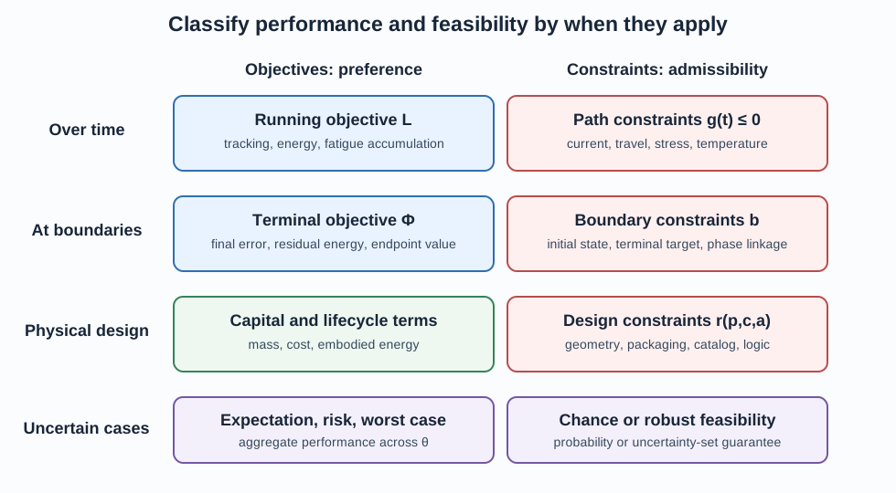
4.6 Path, Boundary, and Physical-Design Constraints
Classify constraints by where they apply ¶ A path constraint must hold throughout an operating interval:
g ( t , x ( t ) , z ( t ) , u ( t ) , p , c , a , d ( t ) ) ≤ 0 ∀ t ∈ [ t 0 , t f ] . g\bigl(t,x(t),z(t),u(t),p,c,a,d(t)\bigr)\le0
\quad \forall t\in[t_0,t_f]. g ( t , x ( t ) , z ( t ) , u ( t ) , p , c , a , d ( t ) ) ≤ 0 ∀ t ∈ [ t 0 , t f ] . For the positioner,
∣ i ( t ) ∣ ≤ i max ( P m ) , ∣ v ( t ) ∣ ≤ v max , ∣ q ( t ) ∣ ≤ q max , T m ( t ) ≤ T max . |i(t)|\le i_{\max}(P_m),\quad
|v(t)|\le v_{\max},\quad
|q(t)|\le q_{\max},\quad
T_m(t)\le T_{\max}. ∣ i ( t ) ∣ ≤ i m a x ( P m ) , ∣ v ( t ) ∣ ≤ v m a x , ∣ q ( t ) ∣ ≤ q m a x , T m ( t ) ≤ T m a x . A boundary constraint applies at the initial or final time, or relates both ends:
q ( t 0 ) = q 0 , ∣ q ( t f ) − r ( t f ) ∣ ≤ ε q , ∣ ω ( t f ) ∣ ≤ ε ω . q(t_0)=q_0,\qquad |q(t_f)-r(t_f)|\le\varepsilon_q,
\qquad |\omega(t_f)|\le\varepsilon_\omega. q ( t 0 ) = q 0 , ∣ q ( t f ) − r ( t f ) ∣ ≤ ε q , ∣ ω ( t f ) ∣ ≤ ε ω . A physical-design constraint depends primarily on time-independent decisions:
m t o t a l ( p , a ) ≤ m max , V e n v e l o p e ( p , a ) ≤ V max , σ ( p ) ≤ σ a l l o w . m_{\mathrm{total}}(p,a)\le m_{\max},\qquad
V_{\mathrm{envelope}}(p,a)\le V_{\max},\qquad
\sigma(p)\le\sigma_{\mathrm{allow}}. m total ( p , a ) ≤ m m a x , V envelope ( p , a ) ≤ V m a x , σ ( p ) ≤ σ allow . Coupling appears in limits ¶ The current limit depends on motor rating, the output-torque limit depends on motor and gear variables, and the terminal error depends on both plant dynamics and control. Separating “plant constraints” from “control constraints” too rigidly can hide these shared dependencies.
Continuous-time verification ¶ A path limit checked only at transcription nodes may be violated between nodes. Reconstruct the continuous trajectory, evaluate constraints on a denser grid, and refine around peaks or switches. For safety-critical limits, include model uncertainty and implementation delay rather than relying on a nominal zero-margin solution.
Activity 4.6: classify each limit ¶ Classify current saturation, final tracking error, gearbox packaging, maximum temperature, zero initial speed, and total mass. Then identify which are coupled plant-control constraints rather than belonging to one discipline alone.
Quantitative audit for Path, Boundary, and Physical-Design Constraints : two complete positioner formulations give the following results.
Formulation RMS error Peak current Dynamic defect Hardware cost A 0.024 rad 11.2 A 3 × 1 0 − 5 3\times10^{-5} 3 × 1 0 − 5 USD 820 B 0.018 rad 13.6 A 8 × 1 0 − 6 8\times10^{-6} 8 × 1 0 − 6 USD 1,050
Use J = e r m s 2 + 1 0 − 5 C J=e_{\rm rms}^2+10^{-5}C J = e rms 2 + 1 0 − 5 C ≤ 14 \leq14 ≤ 14 ≤ 1 0 − 4 \leq10^{-4} ≤ 1 0 − 4
Calculate objectives and constraint margins.
Increase B current by 7% and RMS error by 10% in validation; reassess feasibility and ranking.
Identify which plant, control, state, information, or architecture quantity causes the numerical trade.