Nested Control Co-Design

Nested CCD uses a bi-level structure. The outer optimization chooses plant variables; for each plant candidate, an inner optimization finds its best controller.

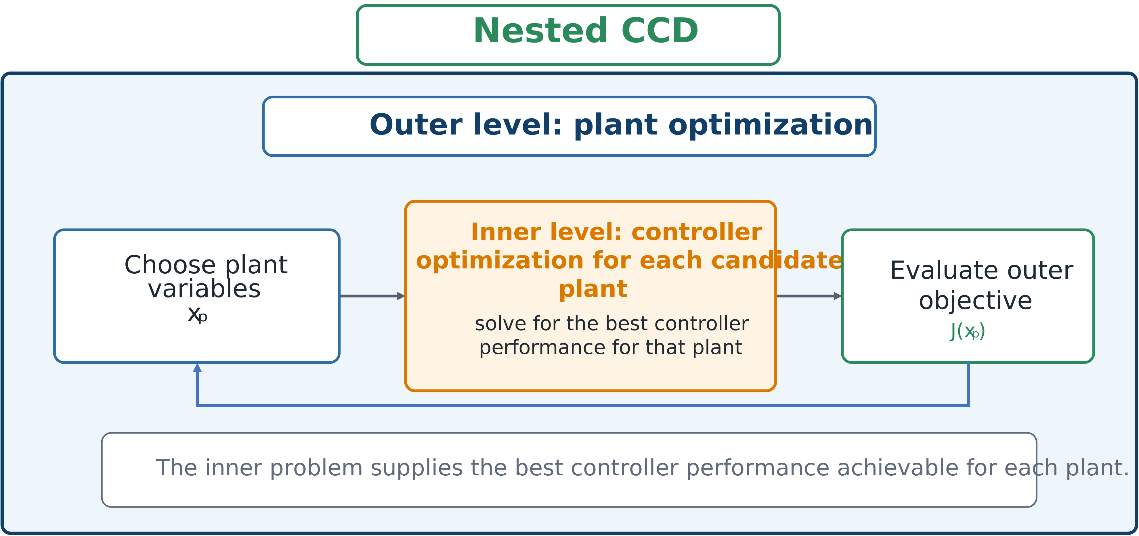
Each plant is evaluated through an inner controller-optimization problem.

An idealized formulation is

subject to the relevant plant, controller, dynamic, and engineering constraints.

The outer loop does not directly choose $\mathbf{x}_c$; it sees the best achievable performance returned by the inner controller solve. This evaluates each plant fairly under the chosen controller structure.

Advantages¶

• Stronger coordination than sequential approaches.

• Natural separation of plant and controller roles.

• Clear interpretation of plant quality under best achievable control.

• Compatibility with established controller-tuning tools.

Limitations¶

Every outer evaluation may require a complete inner optimization. Additional challenges include:

• noise or discontinuity when inner solves are incomplete;

• difficulty differentiating through the inner optimum;

• sensitivity to inner-solver reliability; and

• potentially very high total simulation cost.

Example¶

For active suspension, the outer loop varies stiffness and damping. For each candidate, the inner loop computes optimal feedback gains. The outer loop compares plants using the optimized closed-loop performance returned by the controller solver.

A precise bi-level formulation¶

The idealized statement above hides an important detail: the inner minimization only makes sense if a feasible controller exists for the candidate plant. Write the inner-loop feasible set for a given plant candidate $\mathbf{x}_p^\dagger$ as $\Lambda(\mathbf{x}_p^\dagger)$, the set of controller variables $\mathbf{x}_c$ satisfying the dynamic, path, and boundary constraints associated with that plant. The nested strategy’s induced region is then the set of pairs $(\mathbf{x}_p,\mathbf{x}_c)$ such that $\mathbf{x}_p$ satisfies its own constraints and $\mathbf{x}_c$ minimizes $J(\mathbf{x}_p,\cdot)$ over $\Lambda(\mathbf{x}_p)$.

This induced region is generally a strict subset of the simultaneous problem’s feasible set: a pair $(\mathbf{x}_p,\mathbf{x}_c)$ may satisfy every constraint yet never be produced by the nested strategy if $\mathbf{x}_c$ is feasible but not the optimal response to $\mathbf{x}_p$. For the nested and simultaneous strategies to be equivalent, $\Lambda(\mathbf{x}_p')$ must be nonempty for every plant design $\mathbf{x}_p'$ the outer loop is allowed to propose — otherwise the inner optimization has nothing to return, and the reduced objective $\phi(\mathbf{x}_p')$ is undefined. This “outer-loop feasibility” property is not automatic and, for general co-design problems, is not guaranteed even by classical results such as linear-system controllability once realistic path constraints are present. Practical nested implementations often add an explicit outer-loop feasibility constraint on $\mathbf{x}_p$ so that only plant designs with a workable inner problem are ever offered to the optimizer.

Optimality conditions for the nested strategy¶

The inner controller problem, for a fixed candidate plant, is an ordinary optimal control problem. Adjoining the dynamics and any path constraints with costates $\boldsymbol{\lambda}(t)$ and multipliers $\boldsymbol{\mu}(t)$ forms the Hamiltonian $H=\mathcal{L}+\boldsymbol{\lambda}^T f+\boldsymbol{\mu}^T C$, and Pontryagin’s minimum principle supplies the usual costate dynamics, control stationarity, complementary slackness, and transversality conditions at $t_0$ and $t_f$ — all evaluated at the candidate plant. These conditions are exactly the necessary conditions the inner loop must satisfy.

The outer-loop problem is finite-dimensional in $\mathbf{x}_p$ alone, so its necessary conditions follow from ordinary KKT theory once the total derivative of the reduced objective $\phi(\mathbf{x}_p)=J(\mathbf{x}_p,\mathbf{x}_c^*(\mathbf{x}_p))$ is available:

If the inner problem’s necessary conditions hold exactly, the second term can be shown to vanish by the envelope theorem — Activity 5.4 works through this cancellation explicitly for a quadratic inner problem with an equality-constrained inner solution. In that idealized case, the outer-loop gradient reduces to $\partial J/\partial \mathbf{x}_p$ evaluated along the optimal inner trajectory, and the bookkeeping for $d\mathbf{x}_c^*/d\mathbf{x}_p$ can, in principle, be skipped. In practice this shortcut is dangerous: a numerical inner solver only ever converges to a nonzero optimality or feasibility residual, so the envelope-theorem cancellation is only approximate, and dropping the correction term can silently corrupt the outer-loop gradient. This is the numerical effect Activity 5.4 asks you to quantify directly by sweeping the inner solver’s tolerance.

When the inner problem is a linear-quadratic dynamic optimization problem — quadratic objective, linear time-invariant dynamics, no path constraints, infinite time horizon — the inner loop collapses to a single algebraic Riccati equation, and the optimal feedback gain has the closed form

where $P^*$ is the unique positive-definite solution of $P^*A+A^TP^*-P^*BR^{-1}B^TP^*+Q=0$. This is precisely the structure exploited in Activity 5.3, and it is one of two special inner-loop forms — the other being a general finite-horizon linear-quadratic dynamic optimization problem, solvable after discretization as a convex quadratic program — that make nested CCD attractive in practice: the inner loop can be solved to high accuracy and speed by a tailored algorithm rather than a general-purpose nonlinear optimal control solver.

Activity 5.3: Nested LQR Control Co-Design¶

Activity 5.4: Differentiating a Nested Value Function¶

Activity 5.5: KKT Reformulation of a Constrained Bilevel CCD Problem¶