Variation of the Hamiltonian Integral
the endpoint-variation section derived the first variation of the endpoint portion of the augmented functional. The remaining task is to vary the integral
∫ t 0 t f ( H − λ T x ˙ ) d t , \int_{t_0}^{t_f}\left(H-\boldsymbol{\lambda}^{\mathsf{T}}\dot{\boldsymbol{x}}\right)\,\mathrm{d} t, ∫ t 0 t f ( H − λ T x ˙ ) d t , when the state, control, costate, initial time, and final time are all allowed to vary.
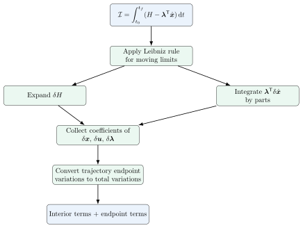
The derivation has four essential steps:
apply the Leibniz rule to account for moving integration limits;
compute the variation of the Hamiltonian;
integrate the term containing δ x ˙ \delta\dot{\boldsymbol{x}} δ x ˙
collect the coefficients of the independent variations.
Starting point ¶ Consider the augmented functional
J a = Φ − ν T ϕ + ∫ t 0 t f ( H − λ T x ˙ ) d t , J_a
=
\Phi-\boldsymbol{\nu}^{\mathsf{T}}\boldsymbol{\phi}
+
\int_{t_0}^{t_f}
\left(H-\boldsymbol{\lambda}^{\mathsf{T}}\dot{\boldsymbol{x}}\right)\,\mathrm{d} t, J a = Φ − ν T ϕ + ∫ t 0 t f ( H − λ T x ˙ ) d t , where
H ( x , u , λ , t ) = L ( x , u , t ) + λ T f ( x , u , t ) . H(\boldsymbol{x},\boldsymbol{u},\boldsymbol{\lambda},t)
=
L(\boldsymbol{x},\boldsymbol{u},t)+\boldsymbol{\lambda}^{\mathsf{T}}\boldsymbol{f}(\boldsymbol{x},\boldsymbol{u},t). H ( x , u , λ , t ) = L ( x , u , t ) + λ T f ( x , u , t ) . The endpoint terms Φ − ν T ϕ \Phi-\boldsymbol{\nu}^{\mathsf{T}}\boldsymbol{\phi} Φ − ν T ϕ
I = ∫ t 0 t f ( H − λ T x ˙ ) d t . \mathcal{I}
=
\int_{t_0}^{t_f}
\left(H-\boldsymbol{\lambda}^{\mathsf{T}}\dot{\boldsymbol{x}}\right)\,\mathrm{d} t. I = ∫ t 0 t f ( H − λ T x ˙ ) d t . This section derives δ I \delta\mathcal{I} δ I
Why t t t ¶ The symbol t t t x ( t ) \boldsymbol{x}(t) x ( t ) u ( t ) \boldsymbol{u}(t) u ( t ) λ ( t ) \boldsymbol{\lambda}(t) λ ( t ) t t t
By contrast, t 0 t_0 t 0 t f t_f t f δ t 0 \delta t_0 δ t 0 δ t f \delta t_f δ t f
Leibniz rule for moving limits ¶ Let
F ( t ) = H ( x , u , λ , t ) − λ T x ˙ . F(t)=H(\boldsymbol{x},\boldsymbol{u},\boldsymbol{\lambda},t)-\boldsymbol{\lambda}^{\mathsf{T}}\dot{\boldsymbol{x}}. F ( t ) = H ( x , u , λ , t ) − λ T x ˙ . Then
I = ∫ t 0 t f F ( t ) d t . \mathcal{I}=\int_{t_0}^{t_f}F(t)\,\mathrm{d} t. I = ∫ t 0 t f F ( t ) d t . The first variation is
δ I = F ( t f ) δ t f − F ( t 0 ) δ t 0 + ∫ t 0 t f δ F ( t ) d t . \delta\mathcal{I}
=
F(t_f)\delta t_f
-
F(t_0)\delta t_0
+
\int_{t_0}^{t_f}\delta F(t)\,\mathrm{d} t. δ I = F ( t f ) δ t f − F ( t 0 ) δ t 0 + ∫ t 0 t f δ F ( t ) d t . Substituting the definition of F F F
δ I = [ H − λ T x ˙ ] t f δ t f − [ H − λ T x ˙ ] t 0 δ t 0 + ∫ t 0 t f δ ( H − λ T x ˙ ) d t . \begin{aligned}
\delta\mathcal{I}
={}&
\left[H-\boldsymbol{\lambda}^{\mathsf{T}}\dot{\boldsymbol{x}}\right]_{t_f}\delta t_f
-
\left[H-\boldsymbol{\lambda}^{\mathsf{T}}\dot{\boldsymbol{x}}\right]_{t_0}\delta t_0
\nonumber\\
&+
\int_{t_0}^{t_f}
\delta\left(H-\boldsymbol{\lambda}^{\mathsf{T}}\dot{\boldsymbol{x}}\right)\,\mathrm{d} t.
\end{aligned} δ I = [ H − λ T x ˙ ] t f δ t f − [ H − λ T x ˙ ] t 0 δ t 0 + ∫ t 0 t f δ ( H − λ T x ˙ ) d t . Variation of the integrand ¶ The integrand variation is
δ ( H − λ T x ˙ ) = δ H − δ ( λ T x ˙ ) . \delta\left(H-\boldsymbol{\lambda}^{\mathsf{T}}\dot{\boldsymbol{x}}\right)
=
\delta H
-
\delta\left(\boldsymbol{\lambda}^{\mathsf{T}}\dot{\boldsymbol{x}}\right). δ ( H − λ T x ˙ ) = δH − δ ( λ T x ˙ ) . Using the product rule,
δ ( λ T x ˙ ) = δ λ T x ˙ + λ T δ x ˙ . \delta\left(\boldsymbol{\lambda}^{\mathsf{T}}\dot{\boldsymbol{x}}\right)
=
\delta\boldsymbol{\lambda}^{\mathsf{T}}\dot{\boldsymbol{x}}
+
\boldsymbol{\lambda}^{\mathsf{T}}\delta\dot{\boldsymbol{x}}. δ ( λ T x ˙ ) = δ λ T x ˙ + λ T δ x ˙ . Therefore,
δ ( H − λ T x ˙ ) = δ H − δ λ T x ˙ − λ T δ x ˙ . \delta\left(H-\boldsymbol{\lambda}^{\mathsf{T}}\dot{\boldsymbol{x}}\right)
=
\delta H
-
\delta\boldsymbol{\lambda}^{\mathsf{T}}\dot{\boldsymbol{x}}
-
\boldsymbol{\lambda}^{\mathsf{T}}\delta\dot{\boldsymbol{x}}. δ ( H − λ T x ˙ ) = δH − δ λ T x ˙ − λ T δ x ˙ . Variation of the Hamiltonian ¶ Because
H = H ( x , u , λ , t ) , H=H(\boldsymbol{x},\boldsymbol{u},\boldsymbol{\lambda},t), H = H ( x , u , λ , t ) , the variation of H H H t t t
δ H = H x δ x + H u δ u + H λ δ λ . \delta H
=
H_{\boldsymbol{x}}\delta\boldsymbol{x}
+
H_{\boldsymbol{u}}\delta\boldsymbol{u}
+
H_{\boldsymbol{\lambda}}\delta\boldsymbol{\lambda}. δH = H x δ x + H u δ u + H λ δ λ . Here the derivative convention is
H x = ∂ H ∂ x ∈ R 1 × n , H u = ∂ H ∂ u ∈ R 1 × m , H λ = ∂ H ∂ λ ∈ R 1 × n . \begin{aligned}
H_{\boldsymbol{x}}&=\frac{\partial H}{\partial\boldsymbol{x}}\in\mathbb{R}^{1\times n},
&H_{\boldsymbol{u}}&=\frac{\partial H}{\partial\boldsymbol{u}}\in\mathbb{R}^{1\times m},
&H_{\boldsymbol{\lambda}}&=\frac{\partial H}{\partial\boldsymbol{\lambda}}\in\mathbb{R}^{1\times n}.
\end{aligned} H x = ∂ x ∂ H ∈ R 1 × n , H u = ∂ u ∂ H ∈ R 1 × m , H λ = ∂ λ ∂ H ∈ R 1 × n . Thus each product in (14)
Substitution into (12)
δ ( H − λ T x ˙ ) = H x δ x + H u δ u + H λ δ λ − δ λ T x ˙ − λ T δ x ˙ . \begin{aligned}
\delta\left(H-\boldsymbol{\lambda}^{\mathsf{T}}\dot{\boldsymbol{x}}\right)
={}&
H_{\boldsymbol{x}}\delta\boldsymbol{x}
+
H_{\boldsymbol{u}}\delta\boldsymbol{u}
+
H_{\boldsymbol{\lambda}}\delta\boldsymbol{\lambda}
\nonumber\\
&-
\delta\boldsymbol{\lambda}^{\mathsf{T}}\dot{\boldsymbol{x}}
-
\boldsymbol{\lambda}^{\mathsf{T}}\delta\dot{\boldsymbol{x}}.
\end{aligned} δ ( H − λ T x ˙ ) = H x δ x + H u δ u + H λ δ λ − δ λ T x ˙ − λ T δ x ˙ . Integration by parts ¶ The final term in (16) δ x \delta\boldsymbol{x} δ x δ x ˙ \delta\dot{\boldsymbol{x}} δ x ˙
∫ t 0 t f λ T δ x ˙ d t = [ λ T δ x ] t 0 t f − ∫ t 0 t f λ ˙ T δ x d t . \int_{t_0}^{t_f}\boldsymbol{\lambda}^{\mathsf{T}}\delta\dot{\boldsymbol{x}}\,\mathrm{d} t
=
\left[\boldsymbol{\lambda}^{\mathsf{T}}\delta\boldsymbol{x}\right]_{t_0}^{t_f}
-
\int_{t_0}^{t_f}\dot{\boldsymbol{\lambda}}^{\mathsf{T}}\delta\boldsymbol{x}\,\mathrm{d} t. ∫ t 0 t f λ T δ x ˙ d t = [ λ T δ x ] t 0 t f − ∫ t 0 t f λ ˙ T δ x d t . Therefore,
− ∫ t 0 t f λ T δ x ˙ d t = − [ λ T δ x ] t 0 t f + ∫ t 0 t f λ ˙ T δ x d t = λ ( t 0 ) T δ x ( t 0 ) − λ ( t f ) T δ x ( t f ) + ∫ t 0 t f λ ˙ T δ x d t . \begin{aligned}
-
\int_{t_0}^{t_f}\boldsymbol{\lambda}^{\mathsf{T}}\delta\dot{\boldsymbol{x}}\,\mathrm{d} t
={}&
-
\left[\boldsymbol{\lambda}^{\mathsf{T}}\delta\boldsymbol{x}\right]_{t_0}^{t_f}
+
\int_{t_0}^{t_f}\dot{\boldsymbol{\lambda}}^{\mathsf{T}}\delta\boldsymbol{x}\,\mathrm{d} t
\nonumber\\
={}&
\boldsymbol{\lambda}(t_0)^{\mathsf{T}}\delta\boldsymbol{x}(t_0)
-
\boldsymbol{\lambda}(t_f)^{\mathsf{T}}\delta\boldsymbol{x}(t_f)
\nonumber\\
&+
\int_{t_0}^{t_f}\dot{\boldsymbol{\lambda}}^{\mathsf{T}}\delta\boldsymbol{x}\,\mathrm{d} t.
\end{aligned} − ∫ t 0 t f λ T δ x ˙ d t = = − [ λ T δ x ] t 0 t f + ∫ t 0 t f λ ˙ T δ x d t λ ( t 0 ) T δ x ( t 0 ) − λ ( t f ) T δ x ( t f ) + ∫ t 0 t f λ ˙ T δ x d t . The minus sign multiplies the entire integration-by-parts result. A reliable procedure is to first integrate ∫ λ T δ x ˙ d t \int\boldsymbol{\lambda}^{\mathsf{T}}\delta\dot{\boldsymbol{x}}\,\mathrm{d} t ∫ λ T δ x ˙ d t
Rearrangement of the interior terms ¶ Substituting (18)
∫ t 0 t f δ ( H − λ T x ˙ ) d t = λ ( t 0 ) T δ x ( t 0 ) − λ ( t f ) T δ x ( t f ) + ∫ t 0 t f [ H x δ x + λ ˙ T δ x + H u δ u + H λ δ λ − δ λ T x ˙ ] d t . \begin{aligned}
\int_{t_0}^{t_f}
\delta\left(H-\boldsymbol{\lambda}^{\mathsf{T}}\dot{\boldsymbol{x}}\right)\,\mathrm{d} t
={}&
\boldsymbol{\lambda}(t_0)^{\mathsf{T}}\delta\boldsymbol{x}(t_0)
-
\boldsymbol{\lambda}(t_f)^{\mathsf{T}}\delta\boldsymbol{x}(t_f)
\nonumber\\
&+
\int_{t_0}^{t_f}
\Big[
H_{\boldsymbol{x}}\delta\boldsymbol{x}
+
\dot{\boldsymbol{\lambda}}^{\mathsf{T}}\delta\boldsymbol{x}
+
H_{\boldsymbol{u}}\delta\boldsymbol{u}
\nonumber\\
&\hspace{4.5em}
+
H_{\boldsymbol{\lambda}}\delta\boldsymbol{\lambda}
-
\delta\boldsymbol{\lambda}^{\mathsf{T}}\dot{\boldsymbol{x}}
\Big]\,\mathrm{d} t.
\end{aligned} ∫ t 0 t f δ ( H − λ T x ˙ ) d t = λ ( t 0 ) T δ x ( t 0 ) − λ ( t f ) T δ x ( t f ) + ∫ t 0 t f [ H x δ x + λ ˙ T δ x + H u δ u + H λ δ λ − δ λ T x ˙ ] d t . The state-variation terms combine directly:
H x δ x + λ ˙ T δ x = ( H x + λ ˙ T ) δ x . H_{\boldsymbol{x}}\delta\boldsymbol{x}+\dot{\boldsymbol{\lambda}}^{\mathsf{T}}\delta\boldsymbol{x}
=
\left(H_{\boldsymbol{x}}+\dot{\boldsymbol{\lambda}}^{\mathsf{T}}\right)\delta\boldsymbol{x}. H x δ x + λ ˙ T δ x = ( H x + λ ˙ T ) δ x . For the costate-variation terms, use the fact that the expression is scalar:
δ λ T x ˙ = x ˙ T δ λ . \delta\boldsymbol{\lambda}^{\mathsf{T}}\dot{\boldsymbol{x}}
=
\dot{\boldsymbol{x}}^{\mathsf{T}}\delta\boldsymbol{\lambda}. δ λ T x ˙ = x ˙ T δ λ . Hence
H λ δ λ − δ λ T x ˙ = ( H λ − x ˙ T ) δ λ . H_{\boldsymbol{\lambda}}\delta\boldsymbol{\lambda}-
\delta\boldsymbol{\lambda}^{\mathsf{T}}\dot{\boldsymbol{x}}
=
\left(H_{\boldsymbol{\lambda}}-\dot{\boldsymbol{x}}^{\mathsf{T}}\right)\delta\boldsymbol{\lambda}. H λ δ λ − δ λ T x ˙ = ( H λ − x ˙ T ) δ λ . Therefore,
∫ t 0 t f δ ( H − λ T x ˙ ) d t = λ ( t 0 ) T δ x ( t 0 ) − λ ( t f ) T δ x ( t f ) + ∫ t 0 t f [ ( H x + λ ˙ T ) δ x + H u δ u + ( H λ − x ˙ T ) δ λ ] d t . \begin{aligned}
\int_{t_0}^{t_f}
\delta\left(H-\boldsymbol{\lambda}^{\mathsf{T}}\dot{\boldsymbol{x}}\right)\,\mathrm{d} t
={}&
\boldsymbol{\lambda}(t_0)^{\mathsf{T}}\delta\boldsymbol{x}(t_0)
-
\boldsymbol{\lambda}(t_f)^{\mathsf{T}}\delta\boldsymbol{x}(t_f)
\nonumber\\
&+
\int_{t_0}^{t_f}
\Big[
\left(H_{\boldsymbol{x}}+\dot{\boldsymbol{\lambda}}^{\mathsf{T}}\right)\delta\boldsymbol{x}
+
H_{\boldsymbol{u}}\delta\boldsymbol{u}
\nonumber\\
&\hspace{5em}
+
\left(H_{\boldsymbol{\lambda}}-\dot{\boldsymbol{x}}^{\mathsf{T}}\right)\delta\boldsymbol{\lambda}
\Big]\,\mathrm{d} t.
\end{aligned} ∫ t 0 t f δ ( H − λ T x ˙ ) d t = λ ( t 0 ) T δ x ( t 0 ) − λ ( t f ) T δ x ( t f ) + ∫ t 0 t f [ ( H x + λ ˙ T ) δ x + H u δ u + ( H λ − x ˙ T ) δ λ ] d t . Complete variation before endpoint conversion ¶ Combining (8) (23)
δ I = [ H − λ T x ˙ ] t f δ t f − [ H − λ T x ˙ ] t 0 δ t 0 + λ ( t 0 ) T δ x ( t 0 ) − λ ( t f ) T δ x ( t f ) + ∫ t 0 t f [ ( H x + λ ˙ T ) δ x + H u δ u + ( H λ − x ˙ T ) δ λ ] d t . \begin{aligned}
\delta\mathcal{I}
={}&
\left[H-\boldsymbol{\lambda}^{\mathsf{T}}\dot{\boldsymbol{x}}\right]_{t_f}\delta t_f
-
\left[H-\boldsymbol{\lambda}^{\mathsf{T}}\dot{\boldsymbol{x}}\right]_{t_0}\delta t_0
\nonumber\\
&+
\boldsymbol{\lambda}(t_0)^{\mathsf{T}}\delta\boldsymbol{x}(t_0)
-
\boldsymbol{\lambda}(t_f)^{\mathsf{T}}\delta\boldsymbol{x}(t_f)
\nonumber\\
&+
\int_{t_0}^{t_f}
\Big[
\left(H_{\boldsymbol{x}}+\dot{\boldsymbol{\lambda}}^{\mathsf{T}}\right)\delta\boldsymbol{x}
+
H_{\boldsymbol{u}}\delta\boldsymbol{u}
\nonumber\\
&\hspace{5em}
+
\left(H_{\boldsymbol{\lambda}}-\dot{\boldsymbol{x}}^{\mathsf{T}}\right)\delta\boldsymbol{\lambda}
\Big]\,\mathrm{d} t.
\end{aligned} δ I = [ H − λ T x ˙ ] t f δ t f − [ H − λ T x ˙ ] t 0 δ t 0 + λ ( t 0 ) T δ x ( t 0 ) − λ ( t f ) T δ x ( t f ) + ∫ t 0 t f [ ( H x + λ ˙ T ) δ x + H u δ u + ( H λ − x ˙ T ) δ λ ] d t . At this stage, the endpoint state variations are the trajectory variations δ x ( t 0 ) \delta\boldsymbol{x}(t_0) δ x ( t 0 ) δ x ( t f ) \delta\boldsymbol{x}(t_f) δ x ( t f ) δ x 0 \delta\boldsymbol{x}_0 δ x 0 δ x f \delta\boldsymbol{x}_f δ x f
Conversion to total endpoint variations ¶ The total endpoint variations satisfy
δ x 0 = δ x ( t 0 ) + x ˙ ( t 0 ) δ t 0 , \begin{aligned}
\delta\boldsymbol{x}_0
&=
\delta\boldsymbol{x}(t_0)+\dot{\boldsymbol{x}}(t_0)\delta t_0,
\end{aligned} δ x 0 = δ x ( t 0 ) + x ˙ ( t 0 ) δ t 0 , δ x f = δ x ( t f ) + x ˙ ( t f ) δ t f . \begin{aligned}
\delta\boldsymbol{x}_f
&=
\delta\boldsymbol{x}(t_f)+\dot{\boldsymbol{x}}(t_f)\delta t_f.
\end{aligned} δ x f = δ x ( t f ) + x ˙ ( t f ) δ t f . Thus,
δ x ( t 0 ) = δ x 0 − x ˙ ( t 0 ) δ t 0 , \begin{aligned}
\delta\boldsymbol{x}(t_0)
&=
\delta\boldsymbol{x}_0-\dot{\boldsymbol{x}}(t_0)\delta t_0,
\end{aligned} δ x ( t 0 ) = δ x 0 − x ˙ ( t 0 ) δ t 0 , δ x ( t f ) = δ x f − x ˙ ( t f ) δ t f . \begin{aligned}
\delta\boldsymbol{x}(t_f)
&=
\delta\boldsymbol{x}_f-\dot{\boldsymbol{x}}(t_f)\delta t_f.
\end{aligned} δ x ( t f ) = δ x f − x ˙ ( t f ) δ t f . Substitute these relations into the boundary terms in (24)
λ ( t 0 ) T δ x ( t 0 ) − λ ( t f ) T δ x ( t f ) = λ ( t 0 ) T δ x 0 − λ ( t 0 ) T x ˙ ( t 0 ) δ t 0 − λ ( t f ) T δ x f + λ ( t f ) T x ˙ ( t f ) δ t f . \begin{aligned}
&\boldsymbol{\lambda}(t_0)^{\mathsf{T}}\delta\boldsymbol{x}(t_0)
-
\boldsymbol{\lambda}(t_f)^{\mathsf{T}}\delta\boldsymbol{x}(t_f)
\nonumber\\
={}&
\boldsymbol{\lambda}(t_0)^{\mathsf{T}}\delta\boldsymbol{x}_0
-
\boldsymbol{\lambda}(t_0)^{\mathsf{T}}\dot{\boldsymbol{x}}(t_0)\delta t_0
\nonumber\\
&-
\boldsymbol{\lambda}(t_f)^{\mathsf{T}}\delta\boldsymbol{x}_f
+
\boldsymbol{\lambda}(t_f)^{\mathsf{T}}\dot{\boldsymbol{x}}(t_f)\delta t_f.
\end{aligned} = λ ( t 0 ) T δ x ( t 0 ) − λ ( t f ) T δ x ( t f ) λ ( t 0 ) T δ x 0 − λ ( t 0 ) T x ˙ ( t 0 ) δ t 0 − λ ( t f ) T δ x f + λ ( t f ) T x ˙ ( t f ) δ t f . Now combine these terms with the Leibniz endpoint contributions. At the final time,
[ H − λ T x ˙ ] t f δ t f + λ ( t f ) T x ˙ ( t f ) δ t f = H ( t f ) δ t f . \begin{aligned}
&\left[H-\boldsymbol{\lambda}^{\mathsf{T}}\dot{\boldsymbol{x}}\right]_{t_f}\delta t_f
+
\boldsymbol{\lambda}(t_f)^{\mathsf{T}}\dot{\boldsymbol{x}}(t_f)\delta t_f
\nonumber\\
&=H(t_f)\delta t_f.
\end{aligned} [ H − λ T x ˙ ] t f δ t f + λ ( t f ) T x ˙ ( t f ) δ t f = H ( t f ) δ t f . At the initial time,
− [ H − λ T x ˙ ] t 0 δ t 0 − λ ( t 0 ) T x ˙ ( t 0 ) δ t 0 = − H ( t 0 ) δ t 0 . \begin{aligned}
&-
\left[H-\boldsymbol{\lambda}^{\mathsf{T}}\dot{\boldsymbol{x}}\right]_{t_0}\delta t_0
-
\boldsymbol{\lambda}(t_0)^{\mathsf{T}}\dot{\boldsymbol{x}}(t_0)\delta t_0
\nonumber\\
&=-H(t_0)\delta t_0.
\end{aligned} − [ H − λ T x ˙ ] t 0 δ t 0 − λ ( t 0 ) T x ˙ ( t 0 ) δ t 0 = − H ( t 0 ) δ t 0 . Therefore, all terms involving λ T x ˙ δ t \boldsymbol{\lambda}^{\mathsf{T}}\dot{\boldsymbol{x}}\delta t λ T x ˙ δ t
Final expression for the integral variation ¶ The first variation of the Hamiltonian integral is
δ I = λ ( t 0 ) T δ x 0 − λ ( t f ) T δ x f − H ( t 0 ) δ t 0 + H ( t f ) δ t f + ∫ t 0 t f [ ( H x + λ ˙ T ) δ x + H u δ u + ( H λ − x ˙ T ) δ λ ] d t . \boxed{
\begin{aligned}
\delta\mathcal{I}
={}&
\boldsymbol{\lambda}(t_0)^{\mathsf{T}}\delta\boldsymbol{x}_0
-
\boldsymbol{\lambda}(t_f)^{\mathsf{T}}\delta\boldsymbol{x}_f
-
H(t_0)\delta t_0
+
H(t_f)\delta t_f
\\
&+
\int_{t_0}^{t_f}
\Big[
\left(H_{\boldsymbol{x}}+\dot{\boldsymbol{\lambda}}^{\mathsf{T}}\right)\delta\boldsymbol{x}
+
H_{\boldsymbol{u}}\delta\boldsymbol{u}
\\
&\hspace{5em}
+
\left(H_{\boldsymbol{\lambda}}-\dot{\boldsymbol{x}}^{\mathsf{T}}\right)\delta\boldsymbol{\lambda}
\Big]\,\mathrm{d} t.
\end{aligned}
} δ I = λ ( t 0 ) T δ x 0 − λ ( t f ) T δ x f − H ( t 0 ) δ t 0 + H ( t f ) δ t f + ∫ t 0 t f [ ( H x + λ ˙ T ) δ x + H u δ u + ( H λ − x ˙ T ) δ λ ] d t . This is the principal result of the chapter.
The variation splits naturally into two groups:
endpoint contributions multiplying δ x 0 \delta\boldsymbol{x}_0 δ x 0 δ x f \delta\boldsymbol{x}_f δ x f δ t 0 \delta t_0 δ t 0 δ t f \delta t_f δ t f
interior contributions multiplying the arbitrary function variations δ x ( t ) \delta\boldsymbol{x}(t) δ x ( t ) δ u ( t ) \delta\boldsymbol{u}(t) δ u ( t ) δ λ ( t ) \delta\boldsymbol{\lambda}(t) δ λ ( t )
The vanishing of the coefficients of the interior variations generates the differential necessary conditions. The endpoint terms later combine with the endpoint-cost variation to produce transversality conditions.
Dimension verification ¶ The dimensions of the interior coefficients are
H x + λ ˙ T ∈ R 1 × n , δ x ∈ R n × 1 , H u ∈ R 1 × m , δ u ∈ R m × 1 , H λ − x ˙ T ∈ R 1 × n , δ λ ∈ R n × 1 . \begin{aligned}
H_{\boldsymbol{x}}+\dot{\boldsymbol{\lambda}}^{\mathsf{T}} &\in\mathbb{R}^{1\times n},
&\delta\boldsymbol{x}&\in\mathbb{R}^{n\times 1},
\\
H_{\boldsymbol{u}}&\in\mathbb{R}^{1\times m},
&\delta\boldsymbol{u}&\in\mathbb{R}^{m\times 1},
\\
H_{\boldsymbol{\lambda}}-\dot{\boldsymbol{x}}^{\mathsf{T}}&\in\mathbb{R}^{1\times n},
&\delta\boldsymbol{\lambda}&\in\mathbb{R}^{n\times 1}.
\end{aligned} H x + λ ˙ T H u H λ − x ˙ T ∈ R 1 × n , ∈ R 1 × m , ∈ R 1 × n , δ x δ u δ λ ∈ R n × 1 , ∈ R m × 1 , ∈ R n × 1 . Each product is scalar, as required. The endpoint products are also scalar:
λ ( t 0 ) T δ x 0 , λ ( t f ) T δ x f , H ( t 0 ) δ t 0 , H ( t f ) δ t f . \boldsymbol{\lambda}(t_0)^{\mathsf{T}}\delta\boldsymbol{x}_0,
\quad
\boldsymbol{\lambda}(t_f)^{\mathsf{T}}\delta\boldsymbol{x}_f,
\quad
H(t_0)\delta t_0,
\quad
H(t_f)\delta t_f. λ ( t 0 ) T δ x 0 , λ ( t f ) T δ x f , H ( t 0 ) δ t 0 , H ( t f ) δ t f . Interior necessary conditions anticipated ¶ Because the interior variations are independent, the coefficients in (32)
H x + λ ˙ T = 0 T , \begin{aligned}
H_{\boldsymbol{x}}+\dot{\boldsymbol{\lambda}}^{\mathsf{T}}&=\boldsymbol{0}^{\mathsf{T}},
\end{aligned} H x + λ ˙ T = 0 T , H u = 0 T , \begin{aligned}
H_{\boldsymbol{u}}&=\boldsymbol{0}^{\mathsf{T}},
\end{aligned} H u = 0 T , H λ − x ˙ T = 0 T . \begin{aligned}
H_{\boldsymbol{\lambda}}-\dot{\boldsymbol{x}}^{\mathsf{T}}&=\boldsymbol{0}^{\mathsf{T}}.
\end{aligned} H λ − x ˙ T = 0 T . Equivalently,
λ ˙ = − H x T , \begin{aligned}
\dot{\boldsymbol{\lambda}}
&=
-
H_{\boldsymbol{x}}^{\mathsf{T}},
\end{aligned} λ ˙ = − H x T , 0 = H u T , \begin{aligned}
\boldsymbol{0}
&=
H_{\boldsymbol{u}}^{\mathsf{T}},
\end{aligned} 0 = H u T , x ˙ = H λ T . \begin{aligned}
\dot{\boldsymbol{x}}
&=
H_{\boldsymbol{\lambda}}^{\mathsf{T}}.
\end{aligned} x ˙ = H λ T . Since
H = L + λ T f , H=L+\boldsymbol{\lambda}^{\mathsf{T}}\boldsymbol{f}, H = L + λ T f , one has
H λ = f T , H_{\boldsymbol{\lambda}}=\boldsymbol{f}^{\mathsf{T}}, H λ = f T , and therefore
x ˙ = H λ T = f . \dot{\boldsymbol{x}}=H_{\boldsymbol{\lambda}}^{\mathsf{T}}=\boldsymbol{f}. x ˙ = H λ T = f . Thus the variation with respect to the costate simply recovers the original state dynamics.
The equation H u = 0 T H_{\boldsymbol{u}}=\boldsymbol{0}^{\mathsf{T}} H u = 0 T
Geometric picture of the derivation ¶ Figure 1: Logical structure of the integral-variation derivation.
Worked symbolic example ¶ Consider the scalar system
x ˙ = a x + b u \dot{x}=ax+bu x ˙ = a x + b u with running cost
L ( x , u ) = 1 2 q x 2 + 1 2 r u 2 . L(x,u)=\frac{1}{2}qx^2+\frac{1}{2}ru^2. L ( x , u ) = 2 1 q x 2 + 2 1 r u 2 . The Hamiltonian is
H = 1 2 q x 2 + 1 2 r u 2 + λ ( a x + b u ) . H
=
\frac{1}{2}qx^2
+
\frac{1}{2}ru^2
+
\lambda(ax+bu). H = 2 1 q x 2 + 2 1 r u 2 + λ ( a x + b u ) . Its derivatives are
H x = q x + a λ , H u = r u + b λ , H λ = a x + b u . \begin{aligned}
H_x&=qx+a\lambda,
\\
H_u&=ru+b\lambda,
\\
H_\lambda&=ax+bu.
\end{aligned} H x H u H λ = q x + aλ , = r u + bλ , = a x + b u . The interior part of the first variation is
∫ t 0 t f [ ( q x + a λ + λ ˙ ) δ x + ( r u + b λ ) δ u + ( a x + b u − x ˙ ) δ λ ] d t . \begin{aligned}
\int_{t_0}^{t_f}
\Big[
(qx+a\lambda+\dot{\lambda})\delta x
+
(ru+b\lambda)\delta u
+
(ax+bu-\dot{x})\delta\lambda
\Big]\,\mathrm{d} t.
\end{aligned} ∫ t 0 t f [ ( q x + aλ + λ ˙ ) δ x + ( r u + bλ ) δ u + ( a x + b u − x ˙ ) δ λ ] d t . The corresponding interior necessary conditions are
x ˙ = a x + b u , λ ˙ = − q x − a λ , 0 = r u + b λ . \begin{aligned}
\dot{x}&=ax+bu,
\\
\dot{\lambda}&=-qx-a\lambda,
\\
0&=ru+b\lambda.
\end{aligned} x ˙ λ ˙ 0 = a x + b u , = − q x − aλ , = r u + bλ . If r > 0 r>0 r > 0
u ∗ = − b r λ . u^*=-\frac{b}{r}\lambda. u ∗ = − r b λ . Connection to the full first variation ¶ the endpoint-variation section obtained
δ ( Φ − ν T ϕ ) = ( Φ x 0 − ν T ϕ x 0 ) δ x 0 + ( Φ t 0 − ν T ϕ t 0 ) δ t 0 + ( Φ x f − ν T ϕ x f ) δ x f + ( Φ t f − ν T ϕ t f ) δ t f − ϕ T δ ν . \begin{aligned}
\delta(\Phi-\boldsymbol{\nu}^{\mathsf{T}}\boldsymbol{\phi})
={}&
\left(\Phi_{\boldsymbol{x}_0}-\boldsymbol{\nu}^{\mathsf{T}}\boldsymbol{\phi}_{\boldsymbol{x}_0}\right)\delta\boldsymbol{x}_0
+
\left(\Phi_{t_0}-\boldsymbol{\nu}^{\mathsf{T}}\boldsymbol{\phi}_{t_0}\right)\delta t_0
\nonumber\\
&+
\left(\Phi_{\boldsymbol{x}_f}-\boldsymbol{\nu}^{\mathsf{T}}\boldsymbol{\phi}_{\boldsymbol{x}_f}\right)\delta\boldsymbol{x}_f
+
\left(\Phi_{t_f}-\boldsymbol{\nu}^{\mathsf{T}}\boldsymbol{\phi}_{t_f}\right)\delta t_f
-
\boldsymbol{\phi}^{\mathsf{T}}\delta\boldsymbol{\nu}.
\end{aligned} δ ( Φ − ν T ϕ ) = ( Φ x 0 − ν T ϕ x 0 ) δ x 0 + ( Φ t 0 − ν T ϕ t 0 ) δ t 0 + ( Φ x f − ν T ϕ x f ) δ x f + ( Φ t f − ν T ϕ t f ) δ t f − ϕ T δ ν . Adding (32)
δ J a = ( Φ x 0 − ν T ϕ x 0 + λ ( t 0 ) T ) δ x 0 + ( Φ t 0 − ν T ϕ t 0 − H ( t 0 ) ) δ t 0 + ( Φ x f − ν T ϕ x f − λ ( t f ) T ) δ x f + ( Φ t f − ν T ϕ t f + H ( t f ) ) δ t f − ϕ T δ ν + ∫ t 0 t f [ ( H x + λ ˙ T ) δ x + H u δ u + ( H λ − x ˙ T ) δ λ ] d t . \begin{aligned}
\delta J_a
={}&
\left(
\Phi_{\boldsymbol{x}_0}
-
\boldsymbol{\nu}^{\mathsf{T}}\boldsymbol{\phi}_{\boldsymbol{x}_0}
+
\boldsymbol{\lambda}(t_0)^{\mathsf{T}}
\right)\delta\boldsymbol{x}_0
\nonumber\\
&+
\left(
\Phi_{t_0}
-
\boldsymbol{\nu}^{\mathsf{T}}\boldsymbol{\phi}_{t_0}
-
H(t_0)
\right)\delta t_0
\nonumber\\
&+
\left(
\Phi_{\boldsymbol{x}_f}
-
\boldsymbol{\nu}^{\mathsf{T}}\boldsymbol{\phi}_{\boldsymbol{x}_f}
-
\boldsymbol{\lambda}(t_f)^{\mathsf{T}}
\right)\delta\boldsymbol{x}_f
\nonumber\\
&+
\left(
\Phi_{t_f}
-
\boldsymbol{\nu}^{\mathsf{T}}\boldsymbol{\phi}_{t_f}
+
H(t_f)
\right)\delta t_f
-
\boldsymbol{\phi}^{\mathsf{T}}\delta\boldsymbol{\nu}
\nonumber\\
&+
\int_{t_0}^{t_f}
\Big[
\left(H_{\boldsymbol{x}}+\dot{\boldsymbol{\lambda}}^{\mathsf{T}}\right)\delta\boldsymbol{x}
+
H_{\boldsymbol{u}}\delta\boldsymbol{u}
+
\left(H_{\boldsymbol{\lambda}}-\dot{\boldsymbol{x}}^{\mathsf{T}}\right)\delta\boldsymbol{\lambda}
\Big]\,\mathrm{d} t.
\end{aligned} δ J a = ( Φ x 0 − ν T ϕ x 0 + λ ( t 0 ) T ) δ x 0 + ( Φ t 0 − ν T ϕ t 0 − H ( t 0 ) ) δ t 0 + ( Φ x f − ν T ϕ x f − λ ( t f ) T ) δ x f + ( Φ t f − ν T ϕ t f + H ( t f ) ) δ t f − ϕ T δ ν + ∫ t 0 t f [ ( H x + λ ˙ T ) δ x + H u δ u + ( H λ − x ˙ T ) δ λ ] d t . This expression is the starting point for the necessary-conditions section, where the state equation, costate equation, stationarity condition, endpoint feasibility condition, and transversality conditions are stated systematically.
Common errors ¶ Varying the dummy variable t t t Only t 0 t_0 t 0 t f t_f t f
Omitting Leibniz terms. Variable limits produce endpoint contributions even before the integrand itself is varied.
Missing the product-rule term. Both δ λ T x ˙ \delta\boldsymbol{\lambda}^{\mathsf{T}}\dot{\boldsymbol{x}} δ λ T x ˙ λ T δ x ˙ \boldsymbol{\lambda}^{\mathsf{T}}\delta\dot{\boldsymbol{x}} λ T δ x ˙
Losing the sign during integration by parts. The leading minus sign acts on both the endpoint term and the remaining integral.
Confusing δ x ( t f ) \delta\boldsymbol{x}(t_f) δ x ( t f ) δ x f \delta\boldsymbol{x}_f δ x f The latter includes the effect of a moving final time.
Using inconsistent row/column derivative conventions. Every coefficient–variation product must be scalar.
Declaring H u = 0 H_{\boldsymbol{u}}=0 H u = 0 Stationarity is an interior condition.
Connection. With endpoint and integral terms assembled, the coefficients of the independent variations can finally be interpreted as the necessary conditions.