First Variation of the Augmented Functional
The previous section introduced the augmented optimal-control functional, the costate vector, the endpoint multiplier, and the Hamiltonian. The next step is to compute the first variation of the augmented functional carefully enough that all endpoint and interior terms are retained.
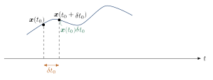
This derivation is delicate for two reasons. First, the initial and final times may vary. Second, the state evaluated at a moving endpoint changes for two distinct reasons: the trajectory may change at a fixed time, and the endpoint time itself may move. Neglecting either contribution produces incorrect transversality conditions.
This section develops the endpoint portion of the derivation and prepares the integral variation that will be completed in the Hamiltonian-integral section.
Problem statement ¶ Consider the optimal-control problem
min x ( ⋅ ) , u ( ⋅ ) , t 0 , t f J = Φ ( x ( t 0 ) , t 0 , x ( t f ) , t f ) + ∫ t 0 t f L ( x ( t ) , u ( t ) , t ) d t , \begin{aligned}
\min_{\boldsymbol{x}(\cdot),\boldsymbol{u}(\cdot),t_0,t_f}\quad
J
&=
\Phi\!\left(\boldsymbol{x}(t_0),t_0,\boldsymbol{x}(t_f),t_f\right)
+
\int_{t_0}^{t_f}
L\!\left(\boldsymbol{x}(t),\boldsymbol{u}(t),t\right)\,\mathrm{d} t,
\end{aligned} x ( ⋅ ) , u ( ⋅ ) , t 0 , t f min J = Φ ( x ( t 0 ) , t 0 , x ( t f ) , t f ) + ∫ t 0 t f L ( x ( t ) , u ( t ) , t ) d t , subject to x ˙ ( t ) = f ( x ( t ) , u ( t ) , t ) , \begin{aligned}
\text{subject to}\quad
\dot{\boldsymbol{x}}(t)
&=
\boldsymbol{f}\!\left(\boldsymbol{x}(t),\boldsymbol{u}(t),t\right),
\end{aligned} subject to x ˙ ( t ) = f ( x ( t ) , u ( t ) , t ) , ϕ ( x ( t 0 ) , t 0 , x ( t f ) , t f ) = 0 . \begin{aligned}
\boldsymbol{\phi}\!\left(\boldsymbol{x}(t_0),t_0,\boldsymbol{x}(t_f),t_f\right)
&=\boldsymbol{0}.
\end{aligned} ϕ ( x ( t 0 ) , t 0 , x ( t f ) , t f ) = 0 . The quantities have dimensions
x ( t ) ∈ R n , u ( t ) ∈ R m , ϕ ∈ R q , λ ( t ) ∈ R n , ν ∈ R q . \begin{aligned}
\boldsymbol{x}(t)&\in\mathbb{R}^n,
&\boldsymbol{u}(t)&\in\mathbb{R}^m,
&\boldsymbol{\phi}&\in\mathbb{R}^q,
&\boldsymbol{\lambda}(t)&\in\mathbb{R}^n,
&\boldsymbol{\nu}&\in\mathbb{R}^q.
\end{aligned} x ( t ) ∈ R n , u ( t ) ∈ R m , ϕ ∈ R q , λ ( t ) ∈ R n , ν ∈ R q . The endpoint function Φ \Phi Φ ϕ \boldsymbol{\phi} ϕ
Augmented functional ¶ Introduce the costate λ ( t ) \boldsymbol{\lambda}(t) λ ( t ) ν \boldsymbol{\nu} ν
J a = Φ ( x ( t 0 ) , t 0 , x ( t f ) , t f ) − ν T ϕ ( x ( t 0 ) , t 0 , x ( t f ) , t f ) + ∫ t 0 t f [ L ( x , u , t ) + λ T ( f ( x , u , t ) − x ˙ ) ] d t . \begin{aligned}
J_a
=
&\Phi\!\left(\boldsymbol{x}(t_0),t_0,\boldsymbol{x}(t_f),t_f\right)
-
\boldsymbol{\nu}^{\mathsf{T}}
\boldsymbol{\phi}\!\left(\boldsymbol{x}(t_0),t_0,\boldsymbol{x}(t_f),t_f\right)
\nonumber\\
&+
\int_{t_0}^{t_f}
\left[
L\!\left(\boldsymbol{x},\boldsymbol{u},t\right)
+
\boldsymbol{\lambda}^{\mathsf{T}}
\left(
\boldsymbol{f}\!\left(\boldsymbol{x},\boldsymbol{u},t\right)-\dot{\boldsymbol{x}}
\right)
\right]
\,\mathrm{d} t.
\end{aligned} J a = Φ ( x ( t 0 ) , t 0 , x ( t f ) , t f ) − ν T ϕ ( x ( t 0 ) , t 0 , x ( t f ) , t f ) + ∫ t 0 t f [ L ( x , u , t ) + λ T ( f ( x , u , t ) − x ˙ ) ] d t . Define the Hamiltonian
H ( x , u , λ , t ) = L ( x , u , t ) + λ T f ( x , u , t ) . H(\boldsymbol{x},\boldsymbol{u},\boldsymbol{\lambda},t)
=
L(\boldsymbol{x},\boldsymbol{u},t)
+
\boldsymbol{\lambda}^{\mathsf{T}}\boldsymbol{f}(\boldsymbol{x},\boldsymbol{u},t). H ( x , u , λ , t ) = L ( x , u , t ) + λ T f ( x , u , t ) . Then
J a = Φ − u v e c T ϕ + ∫ t 0 t f ( H − λ T x ˙ ) d t . J_a
=
\Phi-
uvec^{\mathsf{T}}\boldsymbol{\phi}
+
\int_{t_0}^{t_f}
\left(H-\boldsymbol{\lambda}^{\mathsf{T}}\dot{\boldsymbol{x}}\right)\,\mathrm{d} t. J a = Φ − uv e c T ϕ + ∫ t 0 t f ( H − λ T x ˙ ) d t . Along every feasible trajectory, x ˙ = f \dot{\boldsymbol{x}}=\boldsymbol{f} x ˙ = f ϕ = 0 \boldsymbol{\phi}=\boldsymbol{0} ϕ = 0 J a = J J_a=J J a = J
Moving-endpoint variations ¶ Two distinct endpoint state variations ¶ At the initial endpoint, distinguish
δ x ( t 0 ) \delta\boldsymbol{x}(t_0) δ x ( t 0 ) t 0 t_0 t 0
δ x 0 \delta\boldsymbol{x}_0 δ x 0
These quantities satisfy
δ x 0 = δ x ( t 0 ) + x ˙ ( t 0 ) δ t 0 . \delta\boldsymbol{x}_0
=
\delta\boldsymbol{x}(t_0)
+
\dot{\boldsymbol{x}}(t_0)\delta t_0. δ x 0 = δ x ( t 0 ) + x ˙ ( t 0 ) δ t 0 . Similarly,
δ x f = δ x ( t f ) + x ˙ ( t f ) δ t f . \delta\boldsymbol{x}_f
=
\delta\boldsymbol{x}(t_f)
+
\dot{\boldsymbol{x}}(t_f)\delta t_f. δ x f = δ x ( t f ) + x ˙ ( t f ) δ t f . Equivalently,
δ x ( t 0 ) = δ x 0 − x ˙ ( t 0 ) δ t 0 , \begin{aligned}
\delta\boldsymbol{x}(t_0)
&=
\delta\boldsymbol{x}_0-
\dot{\boldsymbol{x}}(t_0)\delta t_0,
\end{aligned} δ x ( t 0 ) = δ x 0 − x ˙ ( t 0 ) δ t 0 , δ x ( t f ) = δ x f − x ˙ ( t f ) δ t f . \begin{aligned}
\delta\boldsymbol{x}(t_f)
&=
\delta\boldsymbol{x}_f-
\dot{\boldsymbol{x}}(t_f)\delta t_f.
\end{aligned} δ x ( t f ) = δ x f − x ˙ ( t f ) δ t f . Figure 1: A moving endpoint changes the endpoint state through the time shift as well as through a trajectory variation.
Variation of the Mayer cost ¶ Let
Φ = Φ ( x ( t 0 ) , t 0 , x ( t f ) , t f ) . \Phi
=
\Phi\!\left(\boldsymbol{x}(t_0),t_0,\boldsymbol{x}(t_f),t_f\right). Φ = Φ ( x ( t 0 ) , t 0 , x ( t f ) , t f ) . A direct first-order expansion gives
δ Φ = ∂ Φ ∂ x ( t 0 ) δ x ( t 0 ) + ∂ Φ ∂ x ( t 0 ) x ˙ ( t 0 ) δ t 0 + ∂ Φ ∂ t 0 δ t 0 + ∂ Φ ∂ x ( t f ) δ x ( t f ) + ∂ Φ ∂ x ( t f ) x ˙ ( t f ) δ t f + ∂ Φ ∂ t f δ t f . \begin{aligned}
\delta\Phi
=
&\frac{\partial\Phi}{\partial\boldsymbol{x}(t_0)}
\delta\boldsymbol{x}(t_0)
+
\frac{\partial\Phi}{\partial\boldsymbol{x}(t_0)}
\dot{\boldsymbol{x}}(t_0)\delta t_0
+
\frac{\partial\Phi}{\partial t_0}\delta t_0
\nonumber\\
&+
\frac{\partial\Phi}{\partial\boldsymbol{x}(t_f)}
\delta\boldsymbol{x}(t_f)
+
\frac{\partial\Phi}{\partial\boldsymbol{x}(t_f)}
\dot{\boldsymbol{x}}(t_f)\delta t_f
+
\frac{\partial\Phi}{\partial t_f}\delta t_f.
\end{aligned} δ Φ = ∂ x ( t 0 ) ∂ Φ δ x ( t 0 ) + ∂ x ( t 0 ) ∂ Φ x ˙ ( t 0 ) δ t 0 + ∂ t 0 ∂ Φ δ t 0 + ∂ x ( t f ) ∂ Φ δ x ( t f ) + ∂ x ( t f ) ∂ Φ x ˙ ( t f ) δ t f + ∂ t f ∂ Φ δ t f . Using (8) (9)
δ Φ = ∂ Φ ∂ x ( t 0 ) δ x 0 + ∂ Φ ∂ t 0 δ t 0 + ∂ Φ ∂ x ( t f ) δ x f + ∂ Φ ∂ t f δ t f . \boxed{
\delta\Phi
=
\frac{\partial\Phi}{\partial\boldsymbol{x}(t_0)}\delta\boldsymbol{x}_0
+
\frac{\partial\Phi}{\partial t_0}\delta t_0
+
\frac{\partial\Phi}{\partial\boldsymbol{x}(t_f)}\delta\boldsymbol{x}_f
+
\frac{\partial\Phi}{\partial t_f}\delta t_f
}. δ Φ = ∂ x ( t 0 ) ∂ Φ δ x 0 + ∂ t 0 ∂ Φ δ t 0 + ∂ x ( t f ) ∂ Φ δ x f + ∂ t f ∂ Φ δ t f . Orientation convention ¶ Throughout this text, gradients of scalar functions with respect to vectors are taken as row vectors. Thus,
∂ Φ ∂ x ( t 0 ) ∈ R 1 × n , δ x 0 ∈ R n × 1 , \frac{\partial\Phi}{\partial\boldsymbol{x}(t_0)}\in\mathbb{R}^{1\times n},
\qquad
\delta\boldsymbol{x}_0\in\mathbb{R}^{n\times 1}, ∂ x ( t 0 ) ∂ Φ ∈ R 1 × n , δ x 0 ∈ R n × 1 , so their product is scalar.
Variation of the endpoint constraints ¶ The endpoint constraints are
ϕ = ϕ ( x ( t 0 ) , t 0 , x ( t f ) , t f ) ∈ R q . \boldsymbol{\phi}
=
\boldsymbol{\phi}\!\left(\boldsymbol{x}(t_0),t_0,\boldsymbol{x}(t_f),t_f\right)
\in\mathbb{R}^q. ϕ = ϕ ( x ( t 0 ) , t 0 , x ( t f ) , t f ) ∈ R q . Following exactly the same moving-endpoint argument used for Φ \Phi Φ
δ ϕ = ∂ ϕ ∂ x ( t 0 ) δ x 0 + ∂ ϕ ∂ t 0 δ t 0 + ∂ ϕ ∂ x ( t f ) δ x f + ∂ ϕ ∂ t f δ t f . \boxed{
\delta\boldsymbol{\phi}
=
\frac{\partial\boldsymbol{\phi}}{\partial\boldsymbol{x}(t_0)}\delta\boldsymbol{x}_0
+
\frac{\partial\boldsymbol{\phi}}{\partial t_0}\delta t_0
+
\frac{\partial\boldsymbol{\phi}}{\partial\boldsymbol{x}(t_f)}\delta\boldsymbol{x}_f
+
\frac{\partial\boldsymbol{\phi}}{\partial t_f}\delta t_f
}. δ ϕ = ∂ x ( t 0 ) ∂ ϕ δ x 0 + ∂ t 0 ∂ ϕ δ t 0 + ∂ x ( t f ) ∂ ϕ δ x f + ∂ t f ∂ ϕ δ t f . Because ϕ \boldsymbol{\phi} ϕ
∂ ϕ ∂ x ( t 0 ) ∈ R q × n , ∂ ϕ ∂ t 0 ∈ R q × 1 , ∂ ϕ ∂ x ( t f ) ∈ R q × n , ∂ ϕ ∂ t f ∈ R q × 1 . \begin{aligned}
\frac{\partial\boldsymbol{\phi}}{\partial\boldsymbol{x}(t_0)}&\in\mathbb{R}^{q\times n},
&
\frac{\partial\boldsymbol{\phi}}{\partial t_0}&\in\mathbb{R}^{q\times 1},
\\
\frac{\partial\boldsymbol{\phi}}{\partial\boldsymbol{x}(t_f)}&\in\mathbb{R}^{q\times n},
&
\frac{\partial\boldsymbol{\phi}}{\partial t_f}&\in\mathbb{R}^{q\times 1}.
\end{aligned} ∂ x ( t 0 ) ∂ ϕ ∂ x ( t f ) ∂ ϕ ∈ R q × n , ∈ R q × n , ∂ t 0 ∂ ϕ ∂ t f ∂ ϕ ∈ R q × 1 , ∈ R q × 1 . Consequently, every term in (17) R q \mathbb{R}^q R q
Dimension check ¶ For example,
∂ ϕ ∂ x ( t 0 ) ⏟ q × n δ x 0 ⏟ n × 1 ∈ R q × 1 . \underbrace{\frac{\partial\boldsymbol{\phi}}{\partial\boldsymbol{x}(t_0)}}_{q\times n}
\underbrace{\delta\boldsymbol{x}_0}_{n\times 1}
\in\mathbb{R}^{q\times 1}. q × n ∂ x ( t 0 ) ∂ ϕ n × 1 δ x 0 ∈ R q × 1 . Then
ν T ⏟ 1 × q δ ϕ ⏟ q × 1 ∈ R , \underbrace{\boldsymbol{\nu}^{\mathsf{T}}}_{1\times q}
\underbrace{\delta\boldsymbol{\phi}}_{q\times 1}
\in\mathbb{R}, 1 × q ν T q × 1 δ ϕ ∈ R , which is consistent with the fact that ν T ϕ \boldsymbol{\nu}^{\mathsf{T}}\boldsymbol{\phi} ν T ϕ
Variation of the endpoint multiplier term ¶ Apply the product rule to the scalar product ν T ϕ \boldsymbol{\nu}^{\mathsf{T}}\boldsymbol{\phi} ν T ϕ
δ ( ν T ϕ ) = δ ν T ϕ + ν T δ ϕ . \delta\left(\boldsymbol{\nu}^{\mathsf{T}}\boldsymbol{\phi}\right)
=
\delta\boldsymbol{\nu}^{\mathsf{T}}\boldsymbol{\phi}
+
\boldsymbol{\nu}^{\mathsf{T}}\delta\boldsymbol{\phi}. δ ( ν T ϕ ) = δ ν T ϕ + ν T δ ϕ . Therefore,
δ ( − ν T ϕ ) = − δ ν T ϕ − ν T δ ϕ . \delta\left(-\boldsymbol{\nu}^{\mathsf{T}}\boldsymbol{\phi}\right)
=
-\delta\boldsymbol{\nu}^{\mathsf{T}}\boldsymbol{\phi}
-
\boldsymbol{\nu}^{\mathsf{T}}\delta\boldsymbol{\phi}. δ ( − ν T ϕ ) = − δ ν T ϕ − ν T δ ϕ . Substituting (17)
δ ( − ν T ϕ ) = − ν T ∂ ϕ ∂ x ( t 0 ) δ x 0 − ν T ∂ ϕ ∂ t 0 δ t 0 − ν T ∂ ϕ ∂ x ( t f ) δ x f − ν T ∂ ϕ ∂ t f δ t f − δ ν T ϕ . \begin{aligned}
\delta\left(-\boldsymbol{\nu}^{\mathsf{T}}\boldsymbol{\phi}\right)
=
&-\boldsymbol{\nu}^{\mathsf{T}}
\frac{\partial\boldsymbol{\phi}}{\partial\boldsymbol{x}(t_0)}\delta\boldsymbol{x}_0
-
\boldsymbol{\nu}^{\mathsf{T}}
\frac{\partial\boldsymbol{\phi}}{\partial t_0}\delta t_0
\nonumber\\
&-\boldsymbol{\nu}^{\mathsf{T}}
\frac{\partial\boldsymbol{\phi}}{\partial\boldsymbol{x}(t_f)}\delta\boldsymbol{x}_f
-
\boldsymbol{\nu}^{\mathsf{T}}
\frac{\partial\boldsymbol{\phi}}{\partial t_f}\delta t_f
-
\delta\boldsymbol{\nu}^{\mathsf{T}}\boldsymbol{\phi}.
\end{aligned} δ ( − ν T ϕ ) = − ν T ∂ x ( t 0 ) ∂ ϕ δ x 0 − ν T ∂ t 0 ∂ ϕ δ t 0 − ν T ∂ x ( t f ) ∂ ϕ δ x f − ν T ∂ t f ∂ ϕ δ t f − δ ν T ϕ . Because the final term is scalar,
δ ν T ϕ = ϕ T δ ν . \delta\boldsymbol{\nu}^{\mathsf{T}}\boldsymbol{\phi}
=
\boldsymbol{\phi}^{\mathsf{T}}\delta\boldsymbol{\nu}. δ ν T ϕ = ϕ T δ ν . Thus the variation with respect to the endpoint multiplier may be written as
− ϕ T δ ν . -\boldsymbol{\phi}^{\mathsf{T}}\delta\boldsymbol{\nu}. − ϕ T δ ν . Combined endpoint variation ¶ Combine (14) (23)
δ ( Φ − ν T ϕ ) = [ ∂ Φ ∂ x ( t 0 ) − ν T ∂ ϕ ∂ x ( t 0 ) ] δ x 0 + [ ∂ Φ ∂ t 0 − ν T ∂ ϕ ∂ t 0 ] δ t 0 + [ ∂ Φ ∂ x ( t f ) − ν T ∂ ϕ ∂ x ( t f ) ] δ x f + [ ∂ Φ ∂ t f − ν T ∂ ϕ ∂ t f ] δ t f − ϕ T δ ν . \begin{aligned}
\delta\left(\Phi-\boldsymbol{\nu}^{\mathsf{T}}\boldsymbol{\phi}\right)
=
&\left[
\frac{\partial\Phi}{\partial\boldsymbol{x}(t_0)}
-
\boldsymbol{\nu}^{\mathsf{T}}\frac{\partial\boldsymbol{\phi}}{\partial\boldsymbol{x}(t_0)}
\right]\delta\boldsymbol{x}_0
\nonumber\\
&+
\left[
\frac{\partial\Phi}{\partial t_0}
-
\boldsymbol{\nu}^{\mathsf{T}}\frac{\partial\boldsymbol{\phi}}{\partial t_0}
\right]\delta t_0
\nonumber\\
&+
\left[
\frac{\partial\Phi}{\partial\boldsymbol{x}(t_f)}
-
\boldsymbol{\nu}^{\mathsf{T}}\frac{\partial\boldsymbol{\phi}}{\partial\boldsymbol{x}(t_f)}
\right]\delta\boldsymbol{x}_f
\nonumber\\
&+
\left[
\frac{\partial\Phi}{\partial t_f}
-
\boldsymbol{\nu}^{\mathsf{T}}\frac{\partial\boldsymbol{\phi}}{\partial t_f}
\right]\delta t_f
-
\boldsymbol{\phi}^{\mathsf{T}}\delta\boldsymbol{\nu}.
\end{aligned} δ ( Φ − ν T ϕ ) = [ ∂ x ( t 0 ) ∂ Φ − ν T ∂ x ( t 0 ) ∂ ϕ ] δ x 0 + [ ∂ t 0 ∂ Φ − ν T ∂ t 0 ∂ ϕ ] δ t 0 + [ ∂ x ( t f ) ∂ Φ − ν T ∂ x ( t f ) ∂ ϕ ] δ x f + [ ∂ t f ∂ Φ − ν T ∂ t f ∂ ϕ ] δ t f − ϕ T δ ν . This expression should be preserved because it will later be combined with endpoint terms generated by integration by parts in the integral variation.
Define
A 0 T = ∂ Φ ∂ x ( t 0 ) − ν T ∂ ϕ ∂ x ( t 0 ) , B 0 = ∂ Φ ∂ t 0 − ν T ∂ ϕ ∂ t 0 , A f T = ∂ Φ ∂ x ( t f ) − ν T ∂ ϕ ∂ x ( t f ) , B f = ∂ Φ ∂ t f − ν T ∂ ϕ ∂ t f . \begin{aligned}
\boldsymbol{A}_0^{\mathsf{T}}
&=
\frac{\partial\Phi}{\partial\boldsymbol{x}(t_0)}
-
\boldsymbol{\nu}^{\mathsf{T}}\frac{\partial\boldsymbol{\phi}}{\partial\boldsymbol{x}(t_0)},
\\
B_0
&=
\frac{\partial\Phi}{\partial t_0}
-
\boldsymbol{\nu}^{\mathsf{T}}\frac{\partial\boldsymbol{\phi}}{\partial t_0},
\\
\boldsymbol{A}_f^{\mathsf{T}}
&=
\frac{\partial\Phi}{\partial\boldsymbol{x}(t_f)}
-
\boldsymbol{\nu}^{\mathsf{T}}\frac{\partial\boldsymbol{\phi}}{\partial\boldsymbol{x}(t_f)},
\\
B_f
&=
\frac{\partial\Phi}{\partial t_f}
-
\boldsymbol{\nu}^{\mathsf{T}}\frac{\partial\boldsymbol{\phi}}{\partial t_f}.
\end{aligned} A 0 T B 0 A f T B f = ∂ x ( t 0 ) ∂ Φ − ν T ∂ x ( t 0 ) ∂ ϕ , = ∂ t 0 ∂ Φ − ν T ∂ t 0 ∂ ϕ , = ∂ x ( t f ) ∂ Φ − ν T ∂ x ( t f ) ∂ ϕ , = ∂ t f ∂ Φ − ν T ∂ t f ∂ ϕ . Then
δ ( Φ − ν T ϕ ) = A 0 T δ x 0 + B 0 δ t 0 + A f T δ x f + B f δ t f − ϕ T δ ν . \delta\left(\Phi-\boldsymbol{\nu}^{\mathsf{T}}\boldsymbol{\phi}\right)
=
\boldsymbol{A}_0^{\mathsf{T}}\delta\boldsymbol{x}_0
+B_0\delta t_0
+\boldsymbol{A}_f^{\mathsf{T}}\delta\boldsymbol{x}_f
+B_f\delta t_f
-\boldsymbol{\phi}^{\mathsf{T}}\delta\boldsymbol{\nu}. δ ( Φ − ν T ϕ ) = A 0 T δ x 0 + B 0 δ t 0 + A f T δ x f + B f δ t f − ϕ T δ ν . Meaning of the multiplier variation ¶ The variation δ ν \delta\boldsymbol{\nu} δ ν δ ν \delta\boldsymbol{\nu} δ ν
ϕ ( x ( t 0 ) , t 0 , x ( t f ) , t f ) = 0 . \boldsymbol{\phi}\!\left(\boldsymbol{x}(t_0),t_0,\boldsymbol{x}(t_f),t_f\right)=\boldsymbol{0}. ϕ ( x ( t 0 ) , t 0 , x ( t f ) , t f ) = 0 . Thus variation with respect to the multiplier simply recovers the original endpoint constraints.
Whenever a constraint is appended to an objective through a multiplier, variation with respect to the multiplier returns the constraint itself. The role of the multiplier is not to change feasibility, but to allow constrained variations to be represented through an unconstrained stationarity calculation.
Preparation for the integral variation ¶ The remaining part of the augmented functional is
I = ∫ t 0 t f ( H − λ T x ˙ ) d t . I
=
\int_{t_0}^{t_f}
\left(H-\boldsymbol{\lambda}^{\mathsf{T}}\dot{\boldsymbol{x}}\right)\,\mathrm{d} t. I = ∫ t 0 t f ( H − λ T x ˙ ) d t . Its variation must account for
motion of the lower integration limit,
motion of the upper integration limit,
variation of H H H x \boldsymbol{x} x u \boldsymbol{u} u λ \boldsymbol{\lambda} λ
variation of the product λ T x ˙ \boldsymbol{\lambda}^{\mathsf{T}}\dot{\boldsymbol{x}} λ T x ˙
integration by parts of the term containing δ x ˙ \delta\dot{\boldsymbol{x}} δ x ˙
Using Leibniz’s rule,
δ I = ( H − λ T x ˙ ) t f δ t f − ( H − λ T x ˙ ) t 0 δ t 0 + ∫ t 0 t f δ ( H − λ T x ˙ ) d t . \begin{aligned}
\delta I
=
&\left(H-\boldsymbol{\lambda}^{\mathsf{T}}\dot{\boldsymbol{x}}\right)_{t_f}\delta t_f
-
\left(H-\boldsymbol{\lambda}^{\mathsf{T}}\dot{\boldsymbol{x}}\right)_{t_0}\delta t_0
\nonumber\\
&+
\int_{t_0}^{t_f}
\delta\left(H-\boldsymbol{\lambda}^{\mathsf{T}}\dot{\boldsymbol{x}}\right)\,\mathrm{d} t.
\end{aligned} δ I = ( H − λ T x ˙ ) t f δ t f − ( H − λ T x ˙ ) t 0 δ t 0 + ∫ t 0 t f δ ( H − λ T x ˙ ) d t . The interior variation is
δ ( H − λ T x ˙ ) = δ H − δ λ T x ˙ − λ T δ x ˙ . \delta\left(H-\boldsymbol{\lambda}^{\mathsf{T}}\dot{\boldsymbol{x}}\right)
=
\delta H
-
\delta\boldsymbol{\lambda}^{\mathsf{T}}\dot{\boldsymbol{x}}
-
\boldsymbol{\lambda}^{\mathsf{T}}\delta\dot{\boldsymbol{x}}. δ ( H − λ T x ˙ ) = δH − δ λ T x ˙ − λ T δ x ˙ . Furthermore,
δ H = ∂ H ∂ x δ x + ∂ H ∂ u δ u + ∂ H ∂ λ δ λ . \delta H
=
\frac{\partial H}{\partial\boldsymbol{x}}\delta\boldsymbol{x}
+
\frac{\partial H}{\partial\boldsymbol{u}}\delta\boldsymbol{u}
+
\frac{\partial H}{\partial\boldsymbol{\lambda}}\delta\boldsymbol{\lambda}. δH = ∂ x ∂ H δ x + ∂ u ∂ H δ u + ∂ λ ∂ H δ λ . The final term in (32) (26)
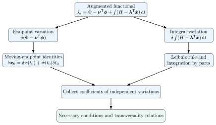
A compact derivation map ¶ Figure 2: Logical structure of the first-variation derivation. This section completes the left branch and prepares the right branch.
Worked symbolic check ¶ Suppose
Φ = 1 2 x ( t f ) T Q f x ( t f ) + α t f , \Phi
=
\frac{1}{2}\boldsymbol{x}(t_f)^{\mathsf{T}} Q_f\boldsymbol{x}(t_f)
+
\alpha t_f, Φ = 2 1 x ( t f ) T Q f x ( t f ) + α t f , where Q f = Q f T ∈ R n × n Q_f=Q_f^{\mathsf{T}}\in\mathbb{R}^{n\times n} Q f = Q f T ∈ R n × n
ϕ = C 0 x ( t 0 ) + C f x ( t f ) − d , \boldsymbol{\phi}
=
C_0\boldsymbol{x}(t_0)+C_f\boldsymbol{x}(t_f)-\boldsymbol{d}, ϕ = C 0 x ( t 0 ) + C f x ( t f ) − d , with C 0 , C f ∈ R q × n C_0,C_f\in\mathbb{R}^{q\times n} C 0 , C f ∈ R q × n
Then
∂ Φ ∂ x ( t 0 ) = 0 T , ∂ Φ ∂ t 0 = 0 , ∂ Φ ∂ x ( t f ) = x ( t f ) T Q f , ∂ Φ ∂ t f = α , \begin{aligned}
\frac{\partial\Phi}{\partial\boldsymbol{x}(t_0)}&=\boldsymbol{0}^{\mathsf{T}},
&
\frac{\partial\Phi}{\partial t_0}&=0,
\\
\frac{\partial\Phi}{\partial\boldsymbol{x}(t_f)}&=\boldsymbol{x}(t_f)^{\mathsf{T}} Q_f,
&
\frac{\partial\Phi}{\partial t_f}&=\alpha,
\end{aligned} ∂ x ( t 0 ) ∂ Φ ∂ x ( t f ) ∂ Φ = 0 T , = x ( t f ) T Q f , ∂ t 0 ∂ Φ ∂ t f ∂ Φ = 0 , = α , and
∂ ϕ ∂ x ( t 0 ) = C 0 , ∂ ϕ ∂ t 0 = 0 , ∂ ϕ ∂ x ( t f ) = C f , ∂ ϕ ∂ t f = 0 . \begin{aligned}
\frac{\partial\boldsymbol{\phi}}{\partial\boldsymbol{x}(t_0)}&=C_0,
&
\frac{\partial\boldsymbol{\phi}}{\partial t_0}&=\boldsymbol{0},
\\
\frac{\partial\boldsymbol{\phi}}{\partial\boldsymbol{x}(t_f)}&=C_f,
&
\frac{\partial\boldsymbol{\phi}}{\partial t_f}&=\boldsymbol{0}.
\end{aligned} ∂ x ( t 0 ) ∂ ϕ ∂ x ( t f ) ∂ ϕ = C 0 , = C f , ∂ t 0 ∂ ϕ ∂ t f ∂ ϕ = 0 , = 0 . Therefore,
δ ( Φ − ν T ϕ ) = − ν T C 0 δ x 0 + ( x ( t f ) T Q f − ν T C f ) δ x f + α δ t f − ϕ T δ ν . \begin{aligned}
\delta(\Phi-\boldsymbol{\nu}^{\mathsf{T}}\boldsymbol{\phi})
=
&-\boldsymbol{\nu}^{\mathsf{T}} C_0\delta\boldsymbol{x}_0
+
\left(\boldsymbol{x}(t_f)^{\mathsf{T}} Q_f-\boldsymbol{\nu}^{\mathsf{T}} C_f\right)\delta\boldsymbol{x}_f
\nonumber\\
&+
\alpha\delta t_f
-
\boldsymbol{\phi}^{\mathsf{T}}\delta\boldsymbol{\nu}.
\end{aligned} δ ( Φ − ν T ϕ ) = − ν T C 0 δ x 0 + ( x ( t f ) T Q f − ν T C f ) δ x f + α δ t f − ϕ T δ ν . This result is dimensionally consistent:
ν T C 0 ∈ R 1 × n , x ( t f ) T Q f ∈ R 1 × n . \boldsymbol{\nu}^{\mathsf{T}} C_0
\in\mathbb{R}^{1\times n},
\qquad
\boldsymbol{x}(t_f)^{\mathsf{T}} Q_f
\in\mathbb{R}^{1\times n}. ν T C 0 ∈ R 1 × n , x ( t f ) T Q f ∈ R 1 × n . Connection. The endpoint calculation is only half of the first variation; the Hamiltonian integral must now be varied with equal care.