Pontryagin’s Necessary Conditions
the preceding two first-variation sections developed the complete first variation of the augmented optimal-control functional. The endpoint terms were expanded carefully, the Hamiltonian integral was varied using the Leibniz rule, and the term containing δ x ˙ \delta\dot{\boldsymbol{x}} δ x ˙
This interpretation produces the equations that every sufficiently regular extremal must satisfy: the state equation, the costate equation, the stationarity or minimum condition, the endpoint constraints, and the transversality conditions. Together, these equations form a coupled two-point boundary-value problem.
Optimal-control problem and augmented functional ¶ Consider the Bolza problem
min u ( ⋅ ) , t 0 , t f J = Φ ( x 0 , t 0 , x f , t f ) + ∫ t 0 t f L ( x , u , t ) d t , \begin{aligned}
\min_{\boldsymbol{u}(\cdot),\,t_0,\,t_f}\quad
J
&=
\Phi\!\left(\boldsymbol{x}_0,t_0,\boldsymbol{x}_f,t_f\right)
+
\int_{t_0}^{t_f}L(\boldsymbol{x},\boldsymbol{u},t)\,\mathrm{d} t,
\end{aligned} u ( ⋅ ) , t 0 , t f min J = Φ ( x 0 , t 0 , x f , t f ) + ∫ t 0 t f L ( x , u , t ) d t , subject to x ˙ = f ( x , u , t ) , \begin{aligned}
\text{subject to}\quad
\dot{\boldsymbol{x}}
&=\boldsymbol{f}(\boldsymbol{x},\boldsymbol{u},t),
\end{aligned} subject to x ˙ = f ( x , u , t ) , ϕ ( x 0 , t 0 , x f , t f ) = 0 , \begin{aligned}
\boldsymbol{\phi}(\boldsymbol{x}_0,t_0,\boldsymbol{x}_f,t_f)
&=\boldsymbol{0},
\end{aligned} ϕ ( x 0 , t 0 , x f , t f ) = 0 , u ( t ) ∈ U ( t ) . \begin{aligned}
\boldsymbol{u}(t)&\in\mathcal{U}(t).
\end{aligned} u ( t ) ∈ U ( t ) . Here, x ( t ) ∈ R n \boldsymbol{x}(t)\in\mathbb{R}^n x ( t ) ∈ R n u ( t ) ∈ R m \boldsymbol{u}(t)\in\mathbb{R}^m u ( t ) ∈ R m ϕ ∈ R q \boldsymbol{\phi}\in\mathbb{R}^q ϕ ∈ R q
The Hamiltonian is
H ( x , u , λ , t ) = L ( x , u , t ) + λ T f ( x , u , t ) , H(\boldsymbol{x},\boldsymbol{u},\boldsymbol{\lambda},t)
=
L(\boldsymbol{x},\boldsymbol{u},t)+\boldsymbol{\lambda}^{\mathsf{T}}\boldsymbol{f}(\boldsymbol{x},\boldsymbol{u},t), H ( x , u , λ , t ) = L ( x , u , t ) + λ T f ( x , u , t ) , and the augmented functional is
J a = Φ − ν T ϕ + ∫ t 0 t f ( H − λ T x ˙ ) d t . J_a
=
\Phi-\boldsymbol{\nu}^{\mathsf{T}}\boldsymbol{\phi}
+
\int_{t_0}^{t_f}
\left(H-\boldsymbol{\lambda}^{\mathsf{T}}\dot{\boldsymbol{x}}\right)\,\mathrm{d} t. J a = Φ − ν T ϕ + ∫ t 0 t f ( H − λ T x ˙ ) d t . The sign convention in (6)
Complete first variation ¶ After the calculations of the preceding two first-variation sections, the first variation can be written as
δ J a = [ Φ x 0 − ν T ϕ x 0 + λ T ( t 0 ) ] δ x 0 + [ Φ t 0 − ν T ϕ t 0 − H ( t 0 ) ] δ t 0 + [ Φ x f − ν T ϕ x f − λ T ( t f ) ] δ x f + [ Φ t f − ν T ϕ t f + H ( t f ) ] δ t f − ϕ T δ ν + ∫ t 0 t f [ H x + λ ˙ T ] δ x d t + ∫ t 0 t f H u δ u d t + ∫ t 0 t f [ H λ − x ˙ T ] δ λ d t . \begin{aligned}
\delta J_a
={}&
\left[
\Phi_{\boldsymbol{x}_0}
-
\boldsymbol{\nu}^{\mathsf{T}}\boldsymbol{\phi}_{\boldsymbol{x}_0}
+
\boldsymbol{\lambda}^{\mathsf{T}}(t_0)
\right]\delta\boldsymbol{x}_0\\
&+
\left[
\Phi_{t_0}
-
\boldsymbol{\nu}^{\mathsf{T}}\boldsymbol{\phi}_{t_0}
-
H(t_0)
\right]\delta t_0
\nonumber\\
&+
\left[
\Phi_{\boldsymbol{x}_f}
-
\boldsymbol{\nu}^{\mathsf{T}}\boldsymbol{\phi}_{\boldsymbol{x}_f}
-
\boldsymbol{\lambda}^{\mathsf{T}}(t_f)
\right]\delta\boldsymbol{x}_f
\nonumber\\
&+
\left[
\Phi_{t_f}
-
\boldsymbol{\nu}^{\mathsf{T}}\boldsymbol{\phi}_{t_f}
+
H(t_f)
\right]\delta t_f
\nonumber\\
&-
\boldsymbol{\phi}^{\mathsf{T}}\delta\boldsymbol{\nu}
\nonumber\\
&+
\int_{t_0}^{t_f}
\left[
H_{\boldsymbol{x}}+\dot{\boldsymbol{\lambda}}^{\mathsf{T}}
\right]\delta\boldsymbol{x}\,\mathrm{d} t
\nonumber\\
&+
\int_{t_0}^{t_f}
H_{\boldsymbol{u}}\delta\boldsymbol{u}\,\mathrm{d} t
\nonumber\\
&+
\int_{t_0}^{t_f}
\left[
H_{\boldsymbol{\lambda}}-\dot{\boldsymbol{x}}^{\mathsf{T}}
\right]\delta\boldsymbol{\lambda}\,\mathrm{d} t.
\nonumber
\end{aligned} δ J a = [ Φ x 0 − ν T ϕ x 0 + λ T ( t 0 ) ] δ x 0 + [ Φ t 0 − ν T ϕ t 0 − H ( t 0 ) ] δ t 0 + [ Φ x f − ν T ϕ x f − λ T ( t f ) ] δ x f + [ Φ t f − ν T ϕ t f + H ( t f ) ] δ t f − ϕ T δ ν + ∫ t 0 t f [ H x + λ ˙ T ] δ x d t + ∫ t 0 t f H u δ u d t + ∫ t 0 t f [ H λ − x ˙ T ] δ λ d t . Subscripts denote row-oriented Jacobians. For example,
H x = ∂ H ∂ x ∈ R 1 × n . H_{\boldsymbol{x}}=\frac{\partial H}{\partial\boldsymbol{x}}\in\mathbb{R}^{1\times n}. H x = ∂ x ∂ H ∈ R 1 × n . Interior necessary conditions ¶ The variations δ x ( t ) \delta\boldsymbol{x}(t) δ x ( t ) δ u ( t ) \delta\boldsymbol{u}(t) δ u ( t ) δ λ ( t ) \delta\boldsymbol{\lambda}(t) δ λ ( t ) ( t 0 , t f ) (t_0,t_f) ( t 0 , t f )
Costate equation ¶ The coefficient of δ x \delta\boldsymbol{x} δ x
H x + λ ˙ T . H_{\boldsymbol{x}}+\dot{\boldsymbol{\lambda}}^{\mathsf{T}}. H x + λ ˙ T . Therefore,
H x + λ ˙ T = 0 T , H_{\boldsymbol{x}}+\dot{\boldsymbol{\lambda}}^{\mathsf{T}}=\boldsymbol{0}^{\mathsf{T}}, H x + λ ˙ T = 0 T , or, equivalently,
λ ˙ = − H x T = − ( ∂ H ∂ x ) T . \boxed{
\dot{\boldsymbol{\lambda}}
=-H_{\boldsymbol{x}}^{\mathsf{T}}
=-\left(\frac{\partial H}{\partial\boldsymbol{x}}\right)^{\mathsf{T}}.
} λ ˙ = − H x T = − ( ∂ x ∂ H ) T . This is called the costate equation or the adjoint equation .
Using (5)
λ ˙ = − L x T − ( f x ) T λ . \dot{\boldsymbol{\lambda}}
=-L_{\boldsymbol{x}}^{\mathsf{T}}
-\left(\boldsymbol{f}_{\boldsymbol{x}}\right)^{\mathsf{T}}\boldsymbol{\lambda}. λ ˙ = − L x T − ( f x ) T λ . Thus, the costate evolves according to both the gradient of the running cost and the local state sensitivity of the dynamics.
State equation recovered from the Hamiltonian ¶ The coefficient of δ λ \delta\boldsymbol{\lambda} δ λ
H λ − x ˙ T = 0 T . H_{\boldsymbol{\lambda}}-\dot{\boldsymbol{x}}^{\mathsf{T}}=\boldsymbol{0}^{\mathsf{T}}. H λ − x ˙ T = 0 T . Therefore,
x ˙ = H λ T . \boxed{
\dot{\boldsymbol{x}}=H_{\boldsymbol{\lambda}}^{\mathsf{T}}.
} x ˙ = H λ T . Since
H = L + λ T f , H=L+\boldsymbol{\lambda}^{\mathsf{T}}\boldsymbol{f}, H = L + λ T f , we have
H λ = f T . H_{\boldsymbol{\lambda}}=\boldsymbol{f}^{\mathsf{T}}. H λ = f T . Hence,
x ˙ = f ( x , u , t ) , \boxed{
\dot{\boldsymbol{x}}=\boldsymbol{f}(\boldsymbol{x},\boldsymbol{u},t),
} x ˙ = f ( x , u , t ) , which is precisely the original state equation. This condition is not new information; it confirms that the augmented formulation enforces the dynamics.
Stationarity condition ¶ For an unconstrained control, or when the optimal control lies in the interior of the admissible set U ( t ) \mathcal{U}(t) U ( t ) δ u \delta\boldsymbol{u} δ u
H u = 0 T . \boxed{
H_{\boldsymbol{u}}=\boldsymbol{0}^{\mathsf{T}}.
} H u = 0 T . Equivalently,
( ∂ H ∂ u ) T = 0 . \left(\frac{\partial H}{\partial\boldsymbol{u}}\right)^{\mathsf{T}}=\boldsymbol{0}. ( ∂ u ∂ H ) T = 0 . If (18)
u ∗ = π ( x , λ , t ) . \boldsymbol{u}^*=\boldsymbol{\pi}(\boldsymbol{x},\boldsymbol{\lambda},t). u ∗ = π ( x , λ , t ) . Substitution into the state and costate equations produces a closed Hamiltonian system in x \boldsymbol{x} x λ \boldsymbol{\lambda} λ
The equation H u = 0 H_{\boldsymbol{u}}=0 H u = 0 u ∗ ( t ) \boldsymbol{u}^*(t) u ∗ ( t ) U ( t ) \mathcal{U}(t) U ( t )
Hamiltonian minimum condition ¶ For a minimization problem with pointwise admissible control set U ( t ) \mathcal{U}(t) U ( t )
H ( x ∗ ( t ) , u ∗ ( t ) , λ ∗ ( t ) , t ) = min u ∈ U ( t ) H ( x ∗ ( t ) , u , λ ∗ ( t ) , t ) . \boxed{
H\bigl(\boldsymbol{x}^*(t),\boldsymbol{u}^*(t),\boldsymbol{\lambda}^*(t),t\bigr)
=
\min_{\boldsymbol{u}\in\mathcal{U}(t)}
H\bigl(\boldsymbol{x}^*(t),\boldsymbol{u},\boldsymbol{\lambda}^*(t),t\bigr).
} H ( x ∗ ( t ) , u ∗ ( t ) , λ ∗ ( t ) , t ) = u ∈ U ( t ) min H ( x ∗ ( t ) , u , λ ∗ ( t ) , t ) . If the minimizing control lies in the interior of U ( t ) \mathcal{U}(t) U ( t ) u \boldsymbol{u} u (21) (18)
For a scalar bounded control,
U = [ u min , u max ] , \mathcal{U}=[u_{\min},u_{\max}], U = [ u m i n , u m a x ] , the minimizer may occur at an endpoint. For example, if
H = a ( t ) u + b ( t ) , H=a(t)u+b(t), H = a ( t ) u + b ( t ) , then
u ∗ ( t ) = { u min , a ( t ) > 0 , u max , a ( t ) < 0 , u^*(t)=
\begin{cases}
u_{\min}, & a(t)>0,\\
u_{\max}, & a(t)<0,
\end{cases} u ∗ ( t ) = { u m i n , u m a x , a ( t ) > 0 , a ( t ) < 0 , with additional analysis required when a ( t ) = 0 a(t)=0 a ( t ) = 0
Endpoint multiplier condition ¶ The multiplier variation appears as
− ϕ T δ ν . -\boldsymbol{\phi}^{\mathsf{T}}\delta\boldsymbol{\nu}. − ϕ T δ ν . Because δ ν \delta\boldsymbol{\nu} δ ν
ϕ ( x 0 , t 0 , x f , t f ) = 0 . \boxed{
\boldsymbol{\phi}(\boldsymbol{x}_0,t_0,\boldsymbol{x}_f,t_f)=\boldsymbol{0}.
} ϕ ( x 0 , t 0 , x f , t f ) = 0 . Thus, variation with respect to the endpoint multiplier recovers the original endpoint constraints.
Transversality conditions ¶ The endpoint variations require more care than the interior variations. An endpoint variable may be fixed, constrained, or free. If it is fixed, its variation is zero and its coefficient need not vanish. If it is free, the variation is arbitrary and the coefficient must vanish.
Initial-state condition ¶ The initial-state contribution is
[ Φ x 0 − ν T ϕ x 0 + λ T ( t 0 ) ] δ x 0 . \left[
\Phi_{\boldsymbol{x}_0}
-
\boldsymbol{\nu}^{\mathsf{T}}\boldsymbol{\phi}_{\boldsymbol{x}_0}
+
\boldsymbol{\lambda}^{\mathsf{T}}(t_0)
\right]\delta\boldsymbol{x}_0. [ Φ x 0 − ν T ϕ x 0 + λ T ( t 0 ) ] δ x 0 . Therefore, either
δ x 0 = 0 , \delta\boldsymbol{x}_0=\boldsymbol{0}, δ x 0 = 0 , or
λ T ( t 0 ) = − Φ x 0 + ν T ϕ x 0 . \boxed{
\boldsymbol{\lambda}^{\mathsf{T}}(t_0)
=-\Phi_{\boldsymbol{x}_0}
+\boldsymbol{\nu}^{\mathsf{T}}\boldsymbol{\phi}_{\boldsymbol{x}_0}.
} λ T ( t 0 ) = − Φ x 0 + ν T ϕ x 0 . In column form,
λ ( t 0 ) = − Φ x 0 T + ϕ x 0 T ν . \boldsymbol{\lambda}(t_0)
=-\Phi_{\boldsymbol{x}_0}^{\mathsf{T}}
+\boldsymbol{\phi}_{\boldsymbol{x}_0}^{\mathsf{T}}\boldsymbol{\nu}. λ ( t 0 ) = − Φ x 0 T + ϕ x 0 T ν . Final-state condition ¶ The final-state contribution is
[ Φ x f − ν T ϕ x f − λ T ( t f ) ] δ x f . \left[
\Phi_{\boldsymbol{x}_f}
-
\boldsymbol{\nu}^{\mathsf{T}}\boldsymbol{\phi}_{\boldsymbol{x}_f}
-
\boldsymbol{\lambda}^{\mathsf{T}}(t_f)
\right]\delta\boldsymbol{x}_f. [ Φ x f − ν T ϕ x f − λ T ( t f ) ] δ x f . Therefore, either
δ x f = 0 , \delta\boldsymbol{x}_f=\boldsymbol{0}, δ x f = 0 , or
λ T ( t f ) = Φ x f − ν T ϕ x f . \boxed{
\boldsymbol{\lambda}^{\mathsf{T}}(t_f)
=
\Phi_{\boldsymbol{x}_f}
-
\boldsymbol{\nu}^{\mathsf{T}}\boldsymbol{\phi}_{\boldsymbol{x}_f}.
} λ T ( t f ) = Φ x f − ν T ϕ x f . In column form,
λ ( t f ) = Φ x f T − ϕ x f T ν . \boldsymbol{\lambda}(t_f)
=
\Phi_{\boldsymbol{x}_f}^{\mathsf{T}}
-\boldsymbol{\phi}_{\boldsymbol{x}_f}^{\mathsf{T}}\boldsymbol{\nu}. λ ( t f ) = Φ x f T − ϕ x f T ν . Initial-time condition ¶ The initial-time contribution is
[ Φ t 0 − ν T ϕ t 0 − H ( t 0 ) ] δ t 0 . \left[
\Phi_{t_0}
-
\boldsymbol{\nu}^{\mathsf{T}}\boldsymbol{\phi}_{t_0}
-
H(t_0)
\right]\delta t_0. [ Φ t 0 − ν T ϕ t 0 − H ( t 0 ) ] δ t 0 . Therefore, either
δ t 0 = 0 , \delta t_0=0, δ t 0 = 0 , or
H ( t 0 ) = Φ t 0 − ν T ϕ t 0 . \boxed{
H(t_0)
=
\Phi_{t_0}
-
\boldsymbol{\nu}^{\mathsf{T}}\boldsymbol{\phi}_{t_0}.
} H ( t 0 ) = Φ t 0 − ν T ϕ t 0 . Final-time condition ¶ The final-time contribution is
[ Φ t f − ν T ϕ t f + H ( t f ) ] δ t f . \left[
\Phi_{t_f}
-
\boldsymbol{\nu}^{\mathsf{T}}\boldsymbol{\phi}_{t_f}
+
H(t_f)
\right]\delta t_f. [ Φ t f − ν T ϕ t f + H ( t f ) ] δ t f . Therefore, either
δ t f = 0 , \delta t_f=0, δ t f = 0 , or
H ( t f ) = − Φ t f + ν T ϕ t f . \boxed{
H(t_f)
=-\Phi_{t_f}
+\boldsymbol{\nu}^{\mathsf{T}}\boldsymbol{\phi}_{t_f}.
} H ( t f ) = − Φ t f + ν T ϕ t f . Fixed and free endpoint cases ¶ Fixed initial state ¶ If x 0 \boldsymbol{x}_0 x 0
δ x 0 = 0 . \delta\boldsymbol{x}_0=\boldsymbol{0}. δ x 0 = 0 . No initial costate condition follows from (7) x ( t 0 ) \boldsymbol{x}(t_0) x ( t 0 ) n n n
Free initial state ¶ If x 0 \boldsymbol{x}_0 x 0 δ x 0 \delta\boldsymbol{x}_0 δ x 0 (29)
Fixed final state ¶ If x f \boldsymbol{x}_f x f
δ x f = 0 . \delta\boldsymbol{x}_f=\boldsymbol{0}. δ x f = 0 . No terminal costate equation is generated by this variation. The prescribed terminal state itself supplies the required boundary information.
Free final state with terminal cost ¶ If x f \boldsymbol{x}_f x f ν \boldsymbol{\nu} ν
λ ( t f ) = Φ x f T . \boxed{
\boldsymbol{\lambda}(t_f)=\Phi_{\boldsymbol{x}_f}^{\mathsf{T}}.
} λ ( t f ) = Φ x f T . If Φ = 0 \Phi=0 Φ = 0
λ ( t f ) = 0 . \boldsymbol{\lambda}(t_f)=\boldsymbol{0}. λ ( t f ) = 0 . Free final time ¶ If t f t_f t f
H ( t f ) + Φ t f = 0. \boxed{
H(t_f)+\Phi_{t_f}=0.
} H ( t f ) + Φ t f = 0. For an autonomous problem with terminal cost independent of time, this becomes
H ( t f ) = 0. H(t_f)=0. H ( t f ) = 0. Endpoint quantity Variation Consequence Fixed x 0 \boldsymbol{x}_0 x 0 δ x 0 = 0 \delta\boldsymbol{x}_0=0 δ x 0 = 0 No condition on λ ( t 0 ) \boldsymbol{\lambda}(t_0) λ ( t 0 ) Free x 0 \boldsymbol{x}_0 x 0 Arbitrary δ x 0 \delta\boldsymbol{x}_0 δ x 0 Apply (29) Fixed x f \boldsymbol{x}_f x f δ x f = 0 \delta\boldsymbol{x}_f=0 δ x f = 0 No terminal costate condition from this variation Free x f \boldsymbol{x}_f x f Arbitrary δ x f \delta\boldsymbol{x}_f δ x f Apply (33) Fixed t 0 t_0 t 0 δ t 0 = 0 \delta t_0=0 δ t 0 = 0 No initial Hamiltonian condition Free t 0 t_0 t 0 Arbitrary δ t 0 \delta t_0 δ t 0 Apply (37) Fixed t f t_f t f δ t f = 0 \delta t_f=0 δ t f = 0 No terminal Hamiltonian condition Free t f t_f t f Arbitrary δ t f \delta t_f δ t f Apply (40)
Common endpoint cases and resulting conditions.
Partial freedom in vector endpoints ¶ A vector endpoint may be partly fixed and partly free. Suppose
x f = [ x f ( F ) x f ( R ) ] , \boldsymbol{x}_f=
\begin{bmatrix}
\boldsymbol{x}_f^{(F)}\\
\boldsymbol{x}_f^{(R)}
\end{bmatrix}, x f = [ x f ( F ) x f ( R ) ] , where x f ( F ) \boldsymbol{x}_f^{(F)} x f ( F ) x f ( R ) \boldsymbol{x}_f^{(R)} x f ( R )
δ x f = [ 0 δ x f ( R ) ] . \delta\boldsymbol{x}_f=
\begin{bmatrix}
\boldsymbol{0}\\
\delta\boldsymbol{x}_f^{(R)}
\end{bmatrix}. δ x f = [ 0 δ x f ( R ) ] . Only the coefficient components associated with δ x f ( R ) \delta\boldsymbol{x}_f^{(R)} δ x f ( R )
Do not label an entire vector endpoint as simply “fixed” or “free” unless all its components share that status. In engineering problems, position may be fixed while velocity, temperature, charge, or orientation remains free.
Hamiltonian system ¶ The state and costate equations form the canonical Hamiltonian system
x ˙ = H λ T , λ ˙ = − H x T . \boxed{
\begin{aligned}
\dot{\boldsymbol{x}}&=H_{\boldsymbol{\lambda}}^{\mathsf{T}},\\
\dot{\boldsymbol{\lambda}}&=-H_{\boldsymbol{x}}^{\mathsf{T}}.
\end{aligned}
} x ˙ λ ˙ = H λ T , = − H x T . When the stationarity condition can be solved for u \boldsymbol{u} u u ∗ = π ( x , λ , t ) \boldsymbol{u}^*=\boldsymbol{\pi}(\boldsymbol{x},\boldsymbol{\lambda},t) u ∗ = π ( x , λ , t )
d d t [ x λ ] = [ H λ T − H x T ] u = π ( x , λ , t ) . \frac{\,\mathrm{d}}{\,\mathrm{d} t}
\begin{bmatrix}
\boldsymbol{x}\\
\boldsymbol{\lambda}
\end{bmatrix}
=
\begin{bmatrix}
H_{\boldsymbol{\lambda}}^{\mathsf{T}}\\
-H_{\boldsymbol{x}}^{\mathsf{T}}
\end{bmatrix}_{\boldsymbol{u}=\boldsymbol{\pi}(\boldsymbol{x},\boldsymbol{\lambda},t)}. d t d [ x λ ] = [ H λ T − H x T ] u = π ( x , λ , t ) . Because both x \boldsymbol{x} x λ \boldsymbol{\lambda} λ n n n 2 n 2n 2 n
Two-point boundary-value structure ¶ The boundary data for (50) t 0 t_0 t 0 t f t_f t f
x ( t 0 ) = x 0 , λ ( t f ) = Φ x f T . \begin{aligned}
\boldsymbol{x}(t_0)&=\boldsymbol{x}_0,\\
\boldsymbol{\lambda}(t_f)&=\Phi_{\boldsymbol{x}_f}^{\mathsf{T}}.
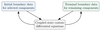
\end{aligned} x ( t 0 ) λ ( t f ) = x 0 , = Φ x f T . The state is specified at the initial time, while the costate is specified at the final time. Therefore, the equations cannot usually be integrated as a conventional initial-value problem.
Figure 1: A general optimality system is a two-point boundary-value problem because boundary information is distributed between the initial and terminal times.
Common numerical approaches include:
single shooting;
multiple shooting;
collocation;
direct transcription;
differential-algebraic boundary-value solvers.
Interpretation of the costate ¶ Let V ( x , t ) V(\boldsymbol{x},t) V ( x , t ) x \boldsymbol{x} x t t t
λ ( t ) = ∇ x V ( x ∗ ( t ) , t ) . \boldsymbol{\lambda}(t)=\nabla_{\boldsymbol{x}}V(\boldsymbol{x}^*(t),t). λ ( t ) = ∇ x V ( x ∗ ( t ) , t ) . Thus, λ i ( t ) \lambda_i(t) λ i ( t ) x i ( t ) x_i(t) x i ( t )
A large positive λ i \lambda_i λ i x i x_i x i x i x_i x i
Conservation of the Hamiltonian ¶ Along a smooth extremal satisfying the state, costate, and stationarity equations,
d H d t = H t . \frac{\,\mathrm{d} H}{\,\mathrm{d} t}
=H_t. d t d H = H t . Therefore, if the problem is autonomous, so that H t = 0 H_t=0 H t = 0
H = constant along the extremal . \boxed{H=\text{constant along the extremal}.} H = constant along the extremal . If, in addition, the final time is free and Φ t f = 0 \Phi_{t_f}=0 Φ t f = 0 H ( t f ) = 0 H(t_f)=0 H ( t f ) = 0
H ( t ) = 0 for all t ∈ [ t 0 , t f ] . H(t)=0
\qquad\text{for all }t\in[t_0,t_f]. H ( t ) = 0 for all t ∈ [ t 0 , t f ] . Worked example: minimum-energy transfer ¶ Consider
min u ( ⋅ ) J = 1 2 ∫ 0 T u 2 ( t ) d t , \begin{aligned}
\min_{u(\cdot)}\quad
J&=\frac{1}{2}\int_0^T u^2(t)\,\mathrm{d} t,
\end{aligned} u ( ⋅ ) min J = 2 1 ∫ 0 T u 2 ( t ) d t , subject to x ˙ = u , \begin{aligned}
\text{subject to}\quad
\dot{x}&=u,
\end{aligned} subject to x ˙ = u , x ( 0 ) = x 0 , x ( T ) = x f , \begin{aligned}
x(0)&=x_0,
\qquad
x(T)=x_f,
\end{aligned} x ( 0 ) = x 0 , x ( T ) = x f , where T T T
The Hamiltonian is
H = 1 2 u 2 + λ u . H=\frac{1}{2}u^2+\lambda u. H = 2 1 u 2 + λ u . The costate equation is
λ ˙ = − H x = 0 , \dot{\lambda}=-H_x=0, λ ˙ = − H x = 0 , so
λ ( t ) = c , \lambda(t)=c, λ ( t ) = c , where c c c
The stationarity condition is
H u = u + λ = 0 , H_u=u+\lambda=0, H u = u + λ = 0 , which gives
u ∗ = − λ = − c . u^*=-\lambda=-c. u ∗ = − λ = − c . Hence,
and
x ( t ) = x 0 − c t . x(t)=x_0-ct. x ( t ) = x 0 − c t . Applying x ( T ) = x f x(T)=x_f x ( T ) = x f
c = x 0 − x f T . c=\frac{x_0-x_f}{T}. c = T x 0 − x f . Therefore,
u ∗ ( t ) = x f − x 0 T , \boxed{
u^*(t)=\frac{x_f-x_0}{T},
} u ∗ ( t ) = T x f − x 0 , and
x ∗ ( t ) = x 0 + x f − x 0 T t . \boxed{
x^*(t)=x_0+\frac{x_f-x_0}{T}t.
} x ∗ ( t ) = x 0 + T x f − x 0 t . The optimal control is constant, and the state moves linearly from x 0 x_0 x 0 x f x_f x f
The terminal state is fixed, so δ x f = 0 \delta x_f=0 δ x f = 0
Worked example: free terminal state ¶ Consider
min u ( ⋅ ) J = 1 2 q ( x ( T ) − x d ) 2 + 1 2 ∫ 0 T r u 2 ( t ) d t , x ˙ = a x + b u , x ( 0 ) = x 0 , \begin{aligned}
\min_{u(\cdot)}\quad
J&=\frac{1}{2}q\bigl(x(T)-x_d\bigr)^2
+\frac{1}{2}\int_0^T r u^2(t)\,\mathrm{d} t,\\
\dot{x}&=a x+b u,\\
x(0)&=x_0,
\end{aligned} u ( ⋅ ) min J x ˙ x ( 0 ) = 2 1 q ( x ( T ) − x d ) 2 + 2 1 ∫ 0 T r u 2 ( t ) d t , = a x + b u , = x 0 , where T T T x ( T ) x(T) x ( T )
The Hamiltonian is
H = 1 2 r u 2 + λ ( a x + b u ) . H=\frac{1}{2}r u^2+\lambda(ax+bu). H = 2 1 r u 2 + λ ( a x + b u ) . The necessary conditions are
x ˙ = a x + b u , λ ˙ = − a λ , 0 = r u + b λ . \begin{aligned}
\dot{x}&=ax+bu,\\
\dot{\lambda}&=-a\lambda,\\
0&=ru+b\lambda.
\end{aligned} x ˙ λ ˙ 0 = a x + b u , = − aλ , = r u + bλ . Thus,
u ∗ = − b r λ . u^*=-\frac{b}{r}\lambda. u ∗ = − r b λ . Because the terminal state is free,
λ ( T ) = Φ x f = q ( x ( T ) − x d ) . \lambda(T)=\Phi_{x_f}
=q\bigl(x(T)-x_d\bigr). λ ( T ) = Φ x f = q ( x ( T ) − x d ) . This terminal condition couples the costate to the terminal tracking error.
Compact statement of the necessary conditions ¶ For a smooth extremal of the problem in (1) (4) λ ( t ) \boldsymbol{\lambda}(t) λ ( t ) ν \boldsymbol{\nu} ν
x ˙ ∗ = H λ T , λ ˙ ∗ = − H x T , u ∗ ( t ) ∈ arg min u ∈ U ( t ) H ( x ∗ , u , λ ∗ , t ) , ϕ ( x 0 , t 0 , x f , t f ) = 0 , \begin{aligned}
\dot{\boldsymbol{x}}^*&=H_{\boldsymbol{\lambda}}^{\mathsf{T}},\\
\dot{\boldsymbol{\lambda}}^*&=-H_{\boldsymbol{x}}^{\mathsf{T}},\\
\boldsymbol{u}^*(t)&\in\arg\min_{\boldsymbol{u}\in\mathcal{U}(t)}H(\boldsymbol{x}^*,\boldsymbol{u},\boldsymbol{\lambda}^*,t),\\
\boldsymbol{\phi}(\boldsymbol{x}_0,t_0,\boldsymbol{x}_f,t_f)&=\boldsymbol{0},
\end{aligned} x ˙ ∗ λ ˙ ∗ u ∗ ( t ) ϕ ( x 0 , t 0 , x f , t f ) = H λ T , = − H x T , ∈ arg u ∈ U ( t ) min H ( x ∗ , u , λ ∗ , t ) , = 0 , together with the transversality conditions corresponding to the endpoint variables that are free.
For interior controls, the minimization condition reduces to
H u = 0 T . H_{\boldsymbol{u}}=\boldsymbol{0}^{\mathsf{T}}. H u = 0 T . A trajectory satisfying the state equation, costate equation, stationarity condition, and transversality conditions is an extremal candidate. These conditions alone do not guarantee a minimum. Second-order conditions, convexity, comparison of candidates, or direct evaluation of the objective may still be required.
Common errors ¶ Imposing a costate condition at a fixed state endpoint. If the endpoint state is fixed, its variation is zero; the corresponding coefficient need not vanish.
Using H u = 0 H_{\boldsymbol{u}}=0 H u = 0 A control on the boundary of its admissible set is determined by Hamiltonian minimization, not necessarily by stationarity.
Losing transposes. Under row-Jacobian conventions, H x H_{\boldsymbol{x}} H x H u H_{\boldsymbol{u}} H u λ ˙ \dot{\boldsymbol{\lambda}} λ ˙ x ˙ \dot{\boldsymbol{x}} x ˙
Confusing δ x ( t f ) \delta\boldsymbol{x}(t_f) δ x ( t f ) δ x f \delta\boldsymbol{x}_f δ x f For moving terminal time, these are related by δ x f = δ x ( t f ) + x ˙ ( t f ) δ t f \delta\boldsymbol{x}_f=\delta\boldsymbol{x}(t_f)+\dot{\boldsymbol{x}}(t_f)\delta t_f δ x f = δ x ( t f ) + x ˙ ( t f ) δ t f
Treating all endpoint components identically. Mixed fixed/free endpoint vectors require componentwise conditions.
Assuming an extremal is automatically optimal. First-order conditions identify candidates only.