Model Fidelity and Surrogate Models

A fidelity ladder¶

No single model is best for every stage. Model fidelity should rise as the design narrows and the claim becomes stronger.

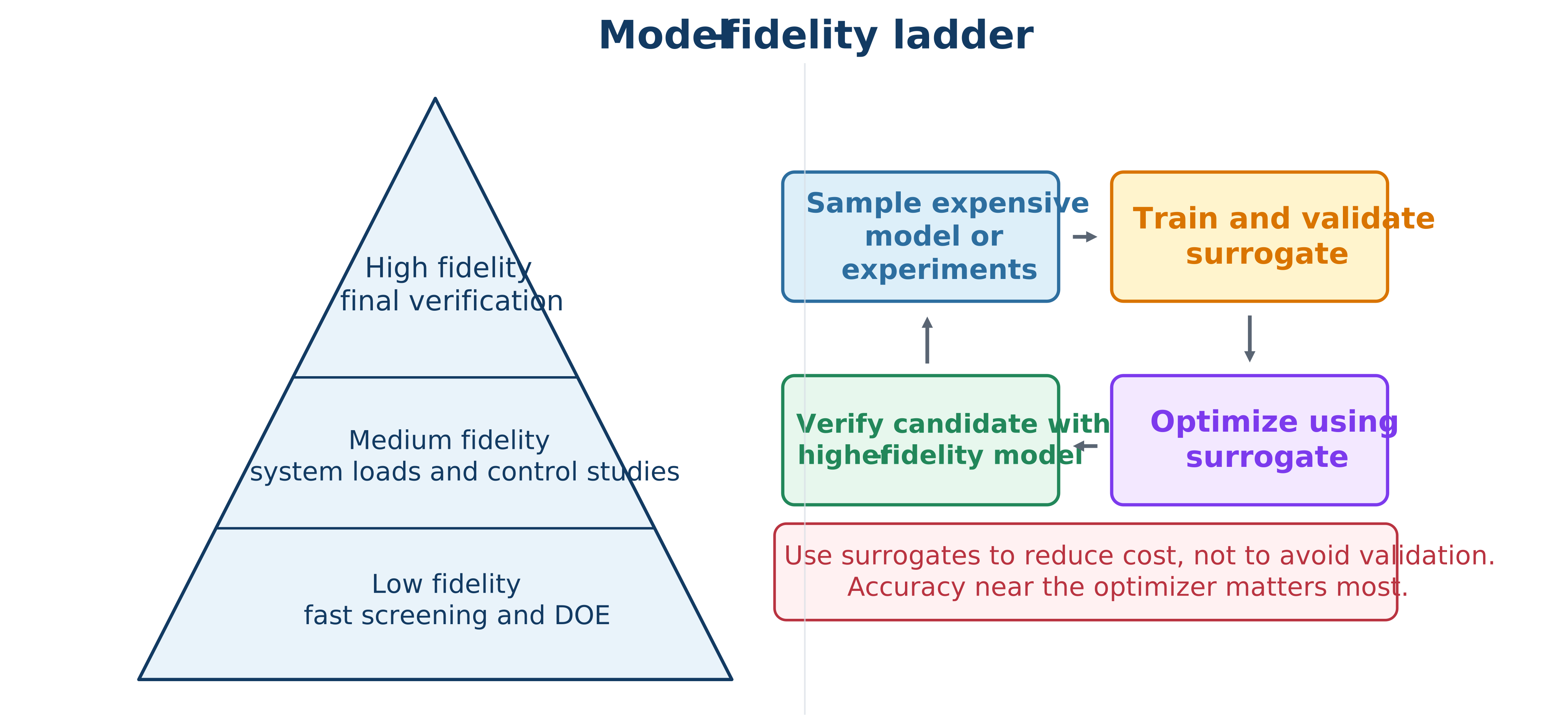
A staged fidelity ladder for practical CCD.

Low fidelity supports broad exploration, sensitivity studies, architecture screening, and initialization.
Medium fidelity adds nonlinearities, actuator and sensor models, realistic loading, and implementation details.
High fidelity provides cross-checks with detailed multiphysics simulation, hardware-in-the-loop (HIL), prototypes, or experiments.

The key question is not whether a model is “accurate” in general, but whether it is sufficiently accurate for the design decision. The optimum can exploit omitted physics, so discrepancy must be assessed near promising designs, not only near a baseline.

Surrogate-assisted CCD¶

When repeated high-fidelity simulations are expensive, a surrogate workflow can:

sample plant, control, and operating variables;
run high-fidelity closed-loop simulations;
fit a reduced-order model, response surface, Gaussian process, neural surrogate, or derivative-function surrogate;
validate within the intended domain;
optimize with the surrogate;
evaluate candidates in the original model; and
add infill samples where error or improvement is large.

Trust regions, error indicators, and conservative margins can reduce damaging extrapolation. A surrogate for a scalar metric may be insufficient for controller design: transient trajectories, stability, peaks, and path constraints can require a dynamic surrogate.

Multi-fidelity reasoning¶

Low-fidelity models can rank designs or provide trends while a smaller number of high-fidelity cases correct bias and validate candidates. A discrepancy model can be written schematically as

y_H(\mathbf{d})=y_L(\mathbf{d})+\delta(\mathbf{d}),

(1)

where $\mathbf{d}$ collects design and operating variables. The correction $\delta$ is useful only within a validated domain and must not conceal structural model errors.

Comparing data-driven low-fidelity approaches: a floating-wind example¶

Not every surrogate needs a physics-based reduced-order structure. A recent comparison for a floating offshore wind turbine (the IEA-15MW reference turbine on a semisubmersible platform, simulated in OpenFAST through the WEIS toolbox with the open-source ROSCO controller) contrasted three data-driven ways of building a low-fidelity closed-loop “plant” for control optimization:

Subspace system identification (the n4sid/SSARX algorithm) fits a discrete-time linear time-invariant state-space model directly from input–output time series, with model order chosen by a sensitivity study.
Deep learning trains a recurrent network (an LSTM layer with a small number of cells and a fully connected output layer) to map inputs to outputs at each time step.
A derivative function surrogate model (DFSM) identifies a continuous-time state-space model whose states are physically meaningful turbine quantities (platform pitch, tower-top displacement, generator speed, and their time derivatives) rather than an abstract identified state, and schedules the state-space matrices on wind speed using a linear parameter-varying (LPV) structure, interpolating between per-wind-speed models identified from simulated time series.

All three low-fidelity models ran far faster than the original high-fidelity simulation, which took nearly 20 minutes per load case: the n4sid model averaged around 2.5 seconds, the DFSM around 25 seconds, and the LSTM around 70 seconds. Simulation speed alone, however, was a poor guide to usefulness. The n4sid model was cheapest to evaluate but had the highest variance in closed-loop response accuracy across load cases — accurate for some, poor for others — partly because its identified states carry no direct physical meaning, which also makes it awkward to extend into a physically scheduled LPV surrogate. The LSTM had lower average error but still showed considerable case-to-case variance and no guaranteed stability. The DFSM balanced simulation time, accuracy, and consistency across load cases better than either alternative, and, unlike the subspace model, could be scheduled meaningfully on wind speed because its states correspond to physical turbine quantities that the LPV weighting can be built around.

The value of a DFSM for control co-design specifically was tested with a small design of experiments over blade-pitch-controller natural frequency and damping ratio, $\mathbf{x}_c=[\omega_{\mathrm{PC}},\zeta_{\mathrm{PC}}]^T$ : a full-factorial sample of 25 controller points, each evaluated at five wind speeds with several turbulent seeds, was run in both the high-fidelity simulator and the DFSM. The full high-fidelity sweep cost roughly 250 CPU-hours; the same sweep using the DFSM cost about 5 CPU-hours — close to a fifty-times speedup — and the DFSM’s predicted tower-base damage-equivalent-load design space had the same qualitative shape and trends as the high-fidelity design space, even though the DFSM underpredicted the absolute load level and was evaluated at controller values it had not been trained on. For early-stage design-space screening, reproducing the shape of a response surface at a fraction of the cost can be more valuable than an unbiased absolute prediction, provided the bias is characterized before the model is trusted for a final decision.

Activity 8.3: Surrogate-Assisted Wind-Turbine CCD with Adaptive Infill¶

Activity 8.3: Surrogate-Assisted Wind-Turbine CCD with Adaptive Infill

Consider a simplified floating-wind CCD problem with plant and controller variables

\mathbf{x}_p= \begin{bmatrix}D_p&K_m&C_m\end{bmatrix}^{T}, \qquad \mathbf{x}_c= \begin{bmatrix}K_{\Omega}&K_{\theta}&K_{\dot{\theta}}\end{bmatrix}^{T},

(2)

where $D_p$ is a platform-dimension parameter and $K_m$ and $C_m$ are effective mooring stiffness and damping parameters. A high-fidelity simulator returns

\mathbf{y}= \begin{bmatrix} P_{\mathrm{mean}}&\theta_{\mathrm{rms}}&M_{\mathrm{tower,max}}&T_{\mathrm{moor,max}} \end{bmatrix}^{T}.

(3)

The system-level objective is

\begin{aligned} J_{\mathrm{HF}}={}&-\frac{P_{\mathrm{mean}}}{P_{\mathrm{ref}}} +0.3\left(\frac{\theta_{\mathrm{rms}}}{\theta_{\mathrm{ref}}}\right)^2\\ &+0.2\left(\frac{M_{\mathrm{tower,max}}}{M_{\mathrm{ref}}}\right)^2 +0.1\left(\frac{T_{\mathrm{moor,max}}}{T_{\mathrm{ref}}}\right)^2 +C_{\mathrm{plant}}(\mathbf{x}_p). \end{aligned}

(4)

Construct a Latin-hypercube design of experiments containing at least 150 plant-controller samples.
Train separate Gaussian-process or radial-basis surrogates for all four outputs.
Split the data into training, validation, and test sets, and report
$R^2,\qquad \mathrm{RMSE},\qquad \max|e|.$
(5)
Formulate the surrogate CCD problem, including high-fidelity output constraints
$M_{\mathrm{tower,max}}\leq M_{\mathrm{allow}}, \qquad T_{\mathrm{moor,max}}\leq T_{\mathrm{allow}}.$
(6)
Solve the surrogate optimization from at least twenty initial guesses.
Evaluate the best five surrogate candidates in the high-fidelity model.
Define a combined infill criterion
$\mathcal{I}(\mathbf{z}) =\widehat{J}(\mathbf{z})-\kappa\sigma_J(\mathbf{z})+\rho V(\mathbf{z}),$
(7)
where $\sigma_J$ is predictive uncertainty and $V$ is a predicted constraint-violation penalty.
Add at least five adaptive infill points per iteration and repeat until the high-fidelity objective changes by less than $0.5\%$ .
Compare the surrogate optimum and final high-fidelity optimum.
Explain why a surrogate that predicts only annual energy or mean power is insufficient when transient loads appear in the constraints.

Activity 8.4: Multi-Fidelity CCD with a Trust-Region Correction Model¶

Activity 8.4: Multi-Fidelity CCD with a Trust-Region Correction Model

Let $J_L(\mathbf{z})$ be a low-fidelity CCD objective and $J_H(\mathbf{z})$ the corresponding high-fidelity objective, where

\mathbf{z}= \begin{bmatrix} \mathbf{x}_p\\ \mathbf{x}_c \end{bmatrix}.

(8)

Define the discrepancy

\delta(\mathbf{z})=J_H(\mathbf{z})-J_L(\mathbf{z}).

(9)

At iteration $k$ , construct the corrected model

m_k(\mathbf{z})=J_L(\mathbf{z})+\widehat{\delta}_k(\mathbf{z}),

(10)

and solve

\min_{\mathbf{z}}\quad m_k(\mathbf{z}) \qquad \text{subject to} \qquad \left\|\mathbf{z}-\mathbf{z}^{(k)}\right\|_2\leq\Delta_k.

(11)

Derive the predicted reduction
$\Delta m_k=m_k(\mathbf{z}^{(k)}) -m_k(\mathbf{z}^{(k)}+\mathbf{s}_k).$
(12)
Derive the actual high-fidelity reduction
$\Delta J_{H,k}=J_H(\mathbf{z}^{(k)}) -J_H(\mathbf{z}^{(k)}+\mathbf{s}_k).$
(13)
Define the trust-region ratio
$\rho_k=\frac{\Delta J_{H,k}}{\Delta m_k}.$
(14)
Propose explicit rules for:
1. accepting or rejecting the trial design;
2. shrinking the trust region; and
3. expanding the trust region.
Implement the method for a low-fidelity suspension or wind model and a higher-fidelity validation model.
Use both additive and multiplicative corrections:
$J_H\approx J_L+\widehat{\delta}, \qquad J_H\approx\widehat{\beta}J_L.$
(15)
Compare the two correction strategies in terms of
$\text{high-fidelity calls}, \quad \text{final objective}, \quad \text{constraint satisfaction}.$
(16)
Determine whether the low-fidelity optimum lies inside a region where the correction model is accurate.
Explain why unconstrained optimization of a corrected surrogate can be unreliable without a trust region or another mechanism that controls extrapolation.