From Optimization to Implementable Hardware

A numerical optimum is an idealized mathematical object. Implementation requires physical dimensions and components, a digital controller, sensor and estimator specifications, real-time software, communications, and safe saturation and fault behavior.

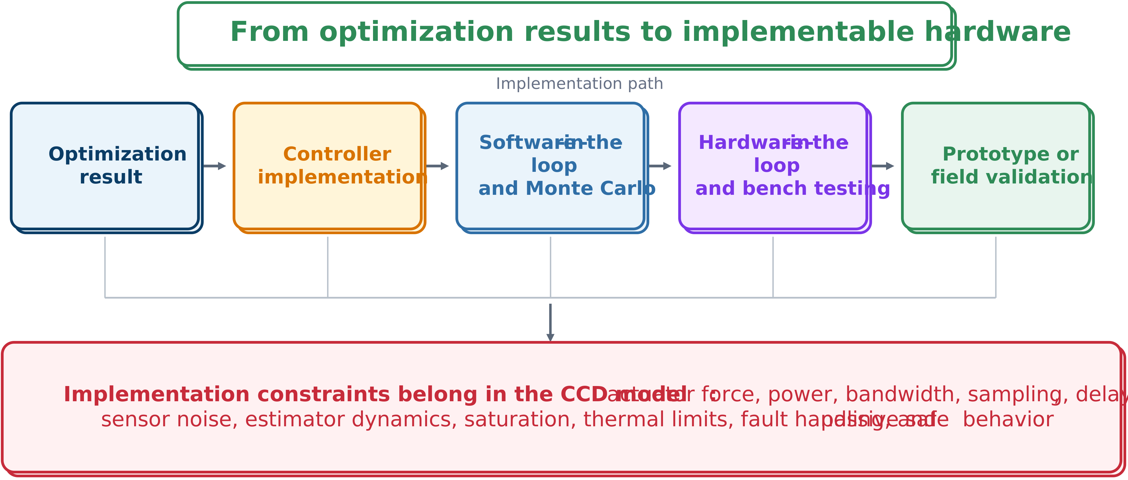
Constraints to model¶

A closed-loop CCD formulation should consider:

• actuator saturation, rate, stroke, bandwidth, and efficiency;

• sampling and computational delay;

• sensor bandwidth, resolution, bias, and noise;

• state-estimation dynamics;

• anti-windup and saturation logic;

• electrical power and thermal limits;

• quantization and communications; and

• behavior when control is disabled.

Controller realization¶

An open-loop optimal trajectory can inform a realizable controller but normally should not be implemented directly unless future inputs are known. Practical transitions include fitting low-order feedback to optimal trajectories, gain scheduling, embedding the problem in MPC, identifying switching or feedforward rules, and simplifying learned policies under explicit safety constraints.

A physical example: from open-loop control to a laboratory MR damper¶

One suspension study made the transition from open-loop optimal control (OLC) trajectories to closed-loop control (CLC) concrete using a physical, reconfigurable trailing-arm suspension testbed whose geometric plant variables could be adjusted on the bench. The design process moved through a sequence of increasingly realistic and increasingly constrained control representations, each solved with the same road input and an objective that minimized sprung-mass acceleration and tire deflection: an unstructured active-force open-loop trajectory gave the best possible, but unrealizable, performance benchmark; a semi-active open-loop damping-force trajectory — assuming an idealized damper able to supply any commanded force at a given velocity — came reasonably close to that benchmark; a semi-active open-loop current trajectory, constrained to the current-versus-force-versus-velocity behavior of a specific, laboratory-characterized magnetorheological (MR) damper, performed measurably worse than the idealized semi-active case because real MR dampers are hysteretic and can only dissipate, not supply, energy; and finally a full-state feedback controller acting on that same MR damper gave the most realizable, but least performant, design in the sequence.

The actuator selected for the physical build was a Lord 8041-1 MR damper, operated over a 0–1 A continuous current range with a maximum stroke of 74 mm. Its force–velocity–current behavior was characterized experimentally in the laboratory and fit with a smooth surrogate model before being used as a hard constraint in both the open-loop and closed-loop problems. Each step in this sequence traded some performance for realizability, and the overall pattern — ideal active, then idealized semi-active, then structured semi-active with a real component model, then closed-loop feedback — is a template for moving any CCD result from an idealized optimal-control benchmark toward a design that can be built and tested.

Validation stages¶

A staged campaign can proceed through:

1. software-in-the-loop simulation;

2. Monte Carlo uncertainty tests;

3. processor-in-the-loop or real-time execution;

4. hardware-in-the-loop testing;

5. component bench tests;

6. scaled or full prototypes; and

7. field validation.

Each stage should address a named modeling or implementation risk and use predefined acceptance criteria.

Activity 8.5: From Optimized Suspension to Implementable Hardware¶