A Quantitative Example
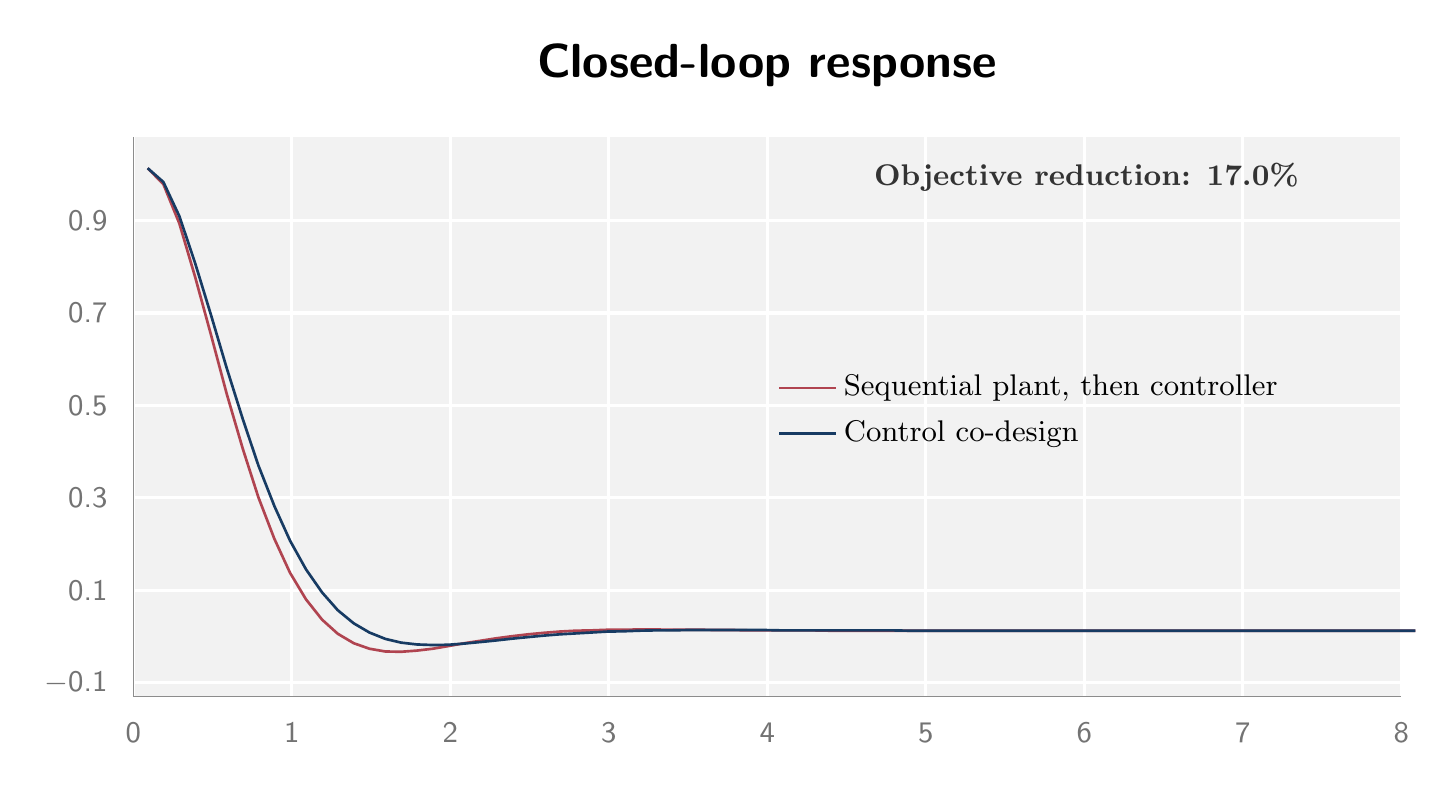
This example compares sequential design and CCD for a mass-spring-damper system. It demonstrates a mechanism, not a universal percentage improvement.
Model and objective
Let and consider the free response from
The plant variables are spring stiffness and passive damping . The controller is
with controller variables and . Define
subject to
The first two integral terms penalize motion, the third penalizes control effort, and the final terms are simplified plant costs.
Two workflows
Sequential workflow
Set and optimize and .
Freeze the resulting plant.
Optimize and for the fixed plant using the full objective.
CCD workflow
Optimize , , , and together using the full objective.
The reported solutions are:
| Method | |||||
|---|---|---|---|---|---|
| Sequential | 2.454 | 1.397 | 5.030 | 2.412 | 0.681 |
| Control co-design | 0.698 | 0.145 | 6.405 | 3.770 | 0.565 |
The co-designed objective is approximately lower:
The important result is not only the lower objective. The optimized plant is different. The CCD solution uses less passive stiffness and damping and relies more on active control. The sequential plant was optimized to perform well without control and retained passive properties that were no longer optimal after the controller was added.
A coupled design landscape. The best controller depends on the plant, and the best plant depends on the controller.
Reproducible implementation
The following Python outline simulates the closed-loop response and evaluates the objective. It can be extended with scipy.optimize.minimize for both workflows.
import numpy as np
from scipy.integrate import solve_ivp

def evaluate(design, t_final=8.0):
    k, c, kp, kd = design

    def dynamics(t, state):
        x, v = state
        u = -kp*x - kd*v
        return [v, -c*v - k*x + u]  # m = 1

    t = np.linspace(0.0, t_final, 2001)
    sol = solve_ivp(dynamics, (0.0, t_final), [1.0, 0.0], t_eval=t,
                    rtol=1e-9, atol=1e-11)
    x, v = sol.y
    u = -kp*x - kd*v

    running_cost = x**2 + 0.05*v**2 + 0.02*u**2
    return np.trapz(running_cost, t) + 0.02*k**2 + 0.03*c**2
For a defensible computational study, report the optimizer, tolerances, initial guesses, bounds, integration grid, convergence status, and constraint residuals. Repeat the optimization from several initial guesses.
Interpreting the result
A co-designed system need not minimize every objective term. It minimizes the selected total objective. Here it accepts greater active-control responsibility in exchange for lower plant cost and a better system-level balance.
This example does not prove that CCD always improves performance by , that software should replace passive hardware, or that the mathematical optimum is ready to build. A realistic study must also address:
actuator saturation, bandwidth, power, and thermal limits;
sensor noise, state estimation, and unmeasured states;
uncertainty, unmodeled dynamics, and disturbance variation;
failure modes and passive-safety requirements;
hardware cost, maintenance, and reliability;
causal real-time implementation; and
higher-fidelity and experimental validation.