Plant-Control Coupling - Control Co-Design

Two groups of decisions are coupled when changing one group changes the best choice in the other. In CCD, the plant changes dynamics, actuator requirements, sensor signals, and achievable performance; the controller changes loads, motions, energy flow, fatigue, and the value of alternative plant designs.

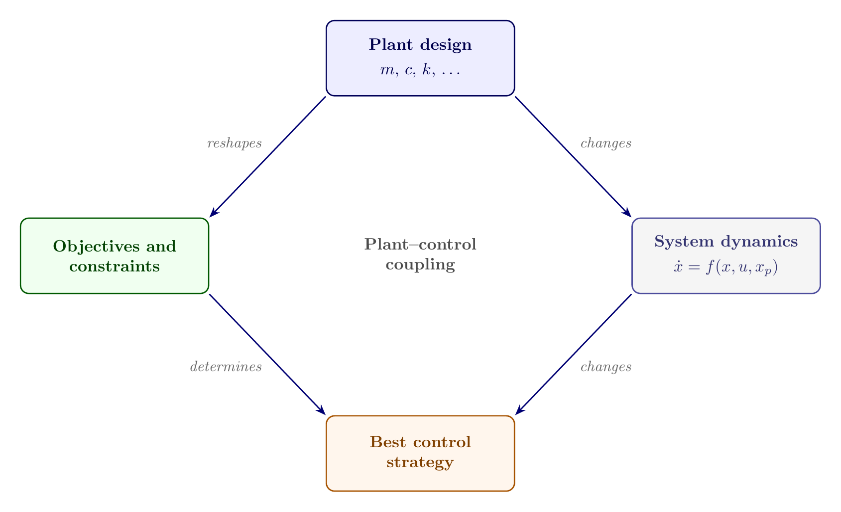
Circular dependence between plant design and controller design. — Plant decisions change the dynamics, the dynamics change the best controller, and controlled behavior changes which plant best serves the mission.

A mass-spring-damper example¶

Consider a mass $m$ , spring $k$ , damper $c$ , actuator force $u(t)$ , and disturbance $d(t)$ :

m\ddot{x}(t)+c\dot{x}(t)+kx(t)=u(t)+d(t).

(1)

With proportional-derivative feedback,

u(t)=-K_px(t)-K_d\dot{x}(t),

(2)

the closed-loop system becomes

m\ddot{x}(t)+(c+K_d)\dot{x}(t)+(k+K_p)x(t)=d(t).

(3)

Passive stiffness $k$ and proportional feedback $K_p$ both contribute to effective closed-loop stiffness. Passive damping $c$ and derivative feedback $K_d$ both contribute to effective damping. They are not interchangeable in practice: active action needs sensors, power, computation, bandwidth, and a functioning actuator. Nevertheless, they can partly substitute for or complement one another.

If $k$ is chosen before $K_p$ is considered, the design may contain more passive stiffness than needed once active control becomes available. If $K_p$ is chosen without plant cost or actuator limits, the controller may demand unrealistic force or energy.

Allocation example¶

Suppose the design requires an effective stiffness

k+K_p=6,

(4)

with normalized cost

C(k,K_p)=0.08k^2+0.02K_p^2.

(5)

A passive-first design sets $K_p=0$ , giving $k=6$ and

C_{\mathrm{seq}}=0.08(6)^2=2.88.

(6)

For co-design, substitute $K_p=6-k$ :

C(k)=0.08k^2+0.02(6-k)^2.

(7)

Setting $dC/dk=0$ yields $k=1.2$ and $K_p=4.8$ , with

C_{\mathrm{CCD}}=0.08(1.2)^2+0.02(4.8)^2=0.576.

(8)

The numbers are deliberately simple. The lesson is general: when passive and active decisions contribute to the same system property, the least-cost allocation may be invisible to a one-pass sequential workflow.

Five ways a plant objective can misrepresent the system¶

The example above hides an important, more general question: when a plant subproblem is optimized on its own, exactly which objective is it optimizing—and how faithfully does that objective represent the true, complete system objective $\phi(\xi(t),u(t),x_p)$ ? Plant-design objectives used in practice fall into five cases, and only two of them are trustworthy:

Case	Accounts for control?	Uses full dynamics?	Objective used
1	No	Yes (passive dynamics)	Exact system objective $\phi(\xi(t),x_p)$
2	No	Yes (passive dynamics)	Approximation $\hat\phi(\xi(t),x_p)$
3	No	No (static analysis)	Approximation $\hat\phi(x_p)$
4	Yes	Yes	Exact system objective $\phi(\xi(t),u(t),x_p)$
5	Yes	Yes	Approximation $\hat\phi(\xi(t),u(t),x_p)$

Case 1 is what “sequential design” means when it is done as well as it can be done without control: the plant is optimized using the real system objective, honestly evaluated with passive dynamics ( $u\equiv0$ ). Case 4 is the true co-design objective: the same real system objective, now evaluated with active control included—this is the objective $J$ inside the compact CCD statement introduced earlier in this chapter. Cases 2, 3, and 5 substitute an approximation $\hat\phi$ for the true objective $\phi$ , most often because building a coupled dynamic model is expensive. Case 3 is the most severe simplification and the most common one in practice: it drops dynamics altogether and uses a static or steady-state proxy—mass, a gravity-balance condition, a frequency-domain margin—standing in for the real, time-dependent performance metric.

In the worked allocation example, the passive-first design implicitly used a Case-3-style objective: it optimized $k$ using a proxy that assumed $K_p=0$ , never evaluating what $K_p$ would eventually need to be. A genuine CCD solution requires a Case 1 or Case 4 objective—the real system objective, honestly evaluated, whether or not active control is present in it.

Common forms of coupling¶

Coupling type	Plant-to-control effect	Control-to-plant effect
Dynamic	Mass, stiffness, damping, geometry, and operating point change the state equations.	Feedback changes effective dynamics, resonance, damping, and transient loads.
Constraint	Plant design changes actuator, temperature, stress, or motion limits.	Control trajectories determine whether stress, fatigue, stroke, and power limits are satisfied.
Economic	Plant size and material alter capital and maintenance cost.	Controller complexity, sensing, computation, and energy use alter lifecycle cost.
Information	Sensor placement and observability change what the controller can know.	Information needs can motivate different sensor locations, structures, or architectures.
Reliability	Passive stability and redundancy alter failure behavior.	Control can reduce loads but introduces hardware, software, and cyber failure modes.
Architecture	Components and connections determine available dynamic pathways.	Desired authority may motivate adding, removing, or relocating components and actuators.

Coupling strength¶

Coupling is strong when a small plant change causes a large change in the optimal controller, or when a small change in control capability causes a large change in the optimal plant. Strong coupling is common when:

active control has substantial authority relative to passive forces;
dynamic behavior dominates performance;
plant constraints depend strongly on state and control trajectories;
multiple time scales or energy domains interact;
control exploits flexible, unstable, resonant, or energy-storing behavior; or
sensing, sampling, delay, or preview limitations influence physical design.

Activity 1.3: Quantifying Plant-Control Coupling¶

Activity 1.3: Quantifying Plant-Control Coupling

Consider the parameterized system-level objective

J(p,c;\gamma) =\frac{1}{2}ap^2+\frac{1}{2}bc^2+\gamma pc-r_pp-r_cc,

(9)

where $a>0$ , $b>0$ , and $\gamma$ represents plant-control coupling strength.

Derive the condition on $\gamma$ for $J$ to be strictly convex.
Derive the optimal controller $c^*(p)$ for a fixed plant.
Compute the controller sensitivity
$\frac{dc^*}{dp}.$
(10)
Derive the optimal plant $p^*(c)$ for a fixed controller and compute
$\frac{dp^*}{dc}.$
(11)
Show that both sensitivities vanish when $\gamma=0$ .
Solve for the simultaneous optimum
$p^*(\gamma), \qquad c^*(\gamma).$
(12)
Use
$a=4, \qquad b=3, \qquad r_p=6, \qquad r_c=5,$
(13)
and evaluate the optimum for
$\gamma\in\{0, 0.5, 1, 2, 3\}.$
(14)
Plot
$\left|\frac{dc^*}{dp}\right|$
(15)
and the sequential performance loss as functions of $\gamma$ .
Propose a dimensionless coupling index based on the Hessian cross-term and justify your choice.

Activity 1.4: Control Authority and the Value of Integration¶

Activity 1.4: Control Authority and the Value of Integration

Consider

m\ddot{x}+c\dot{x}+kx=u,

(16)

with

m=1, \qquad x(0)=1, \qquad \dot{x}(0)=0.

(17)

Use the PD controller

u=-K_px-K_d\dot{x}, \qquad 0\leq K_p\leq K_{p,\max}, \qquad 0\leq K_d\leq K_{d,\max},

(18)

with plant-design bounds

0.1\leq k\leq6, \qquad 0.05\leq c\leq3.

(19)

Define

A_{\mathrm{cl}}= \begin{bmatrix} 0&1\\ -(k+K_p)&-(c+K_d) \end{bmatrix}.

(20)

For stable designs, let $P$ solve

A_{\mathrm{cl}}^TP+PA_{\mathrm{cl}}+Q+K^TRK=0,

(21)

where

Q= \begin{bmatrix} 1&0\\0&0.05 \end{bmatrix}, \qquad R=0.02, \qquad K=\begin{bmatrix}K_p&K_d\end{bmatrix}.

(22)

Define the total cost

J=\mathbf{x}_0^TP\mathbf{x}_0+0.02k^2+0.03c^2, \qquad \mathbf{x}_0= \begin{bmatrix}1\\0\end{bmatrix}.

(23)

Derive the closed-loop stability conditions.
Explain why $\mathbf{x}_0^TP\mathbf{x}_0$ equals the infinite-horizon dynamic performance cost.
For
$K_{p,\max}=K_{d,\max}\in\{0, 0.5, 1, 2, 4, 8\},$
(24)
solve:
1. the passive-first sequential problem; and
2. the simultaneous CCD problem.
Plot the relative CCD advantage
$\eta_{\mathrm{CCD}}= \frac{J_{\mathrm{seq}}-J_{\mathrm{CCD}}}{J_{\mathrm{seq}}}$
(25)
against allowable control authority.
Determine whether the coupling becomes weak as the allowable controller gains approach zero.
Determine whether unlimited control authority drives the optimal passive stiffness and damping to their lower bounds.
Add the actuator-effort regularization
$\beta(K_p^2+K_d^2), \qquad \beta\in\{0, 10^{-3}, 10^{-2}, 10^{-1}\},$
(26)
and repeat the study.
Explain why strong control authority does not automatically imply that the most active design is the most practical design.