Bilinear Tangent Steering Law for Fixed-Time Ascent
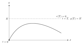
This section develops an analytical optimal control solution for a fixed-time planar steering problem. The objective is to steer an accelerating object from the origin to a prescribed terminal altitude while maximizing its terminal horizontal velocity and forcing the terminal vertical velocity to zero.
The example illustrates several central ideas:
conversion of a maximization problem into minimization form;
Hamiltonian construction;
costate integration;
transversality conditions;
analytical recovery of the optimal steering law;
interpretation of a bilinear tangent law;
explicit integration of the state equations.
Problem Statement ¶ Consider the planar dynamics
x ˙ = u , y ˙ = v , u ˙ = a cos β , v ˙ = a sin β , \begin{aligned}
\dot{x} &= u,\\
\dot{y} &= v,\\
\dot{u} &= a\cos\beta,\\
\dot{v} &= a\sin\beta,
\end{aligned} x ˙ y ˙ u ˙ v ˙ = u , = v , = a cos β , = a sin β , where:
x ( t ) x(t) x ( t )
y ( t ) y(t) y ( t )
u ( t ) u(t) u ( t )
v ( t ) v(t) v ( t )
a a a
β ( t ) \beta(t) β ( t )
The final time T T T
The initial conditions are
x ( 0 ) = 0 , y ( 0 ) = 0 , u ( 0 ) = 0 , v ( 0 ) = 0. x(0)=0,\qquad
y(0)=0,\qquad
u(0)=0,\qquad
v(0)=0. x ( 0 ) = 0 , y ( 0 ) = 0 , u ( 0 ) = 0 , v ( 0 ) = 0. The terminal conditions are
y ( T ) = H , v ( T ) = 0. y(T)=H,
\qquad
v(T)=0. y ( T ) = H , v ( T ) = 0. The terminal horizontal position x ( T ) x(T) x ( T ) u ( T ) u(T) u ( T )
The objective is
max β ( ⋅ ) u ( T ) . \max_{\beta(\cdot)} u(T). β ( ⋅ ) max u ( T ) . Equivalently,
min β ( ⋅ ) Φ = − u ( T ) . \boxed{
\min_{\beta(\cdot)} \Phi=-u(T).
} β ( ⋅ ) min Φ = − u ( T ) . Physical Interpretation ¶ The acceleration vector has constant magnitude a a a β \beta β
a = a [ cos β sin β ] . \boldsymbol{a}
=
a
\begin{bmatrix}
\cos\beta\\
\sin\beta
\end{bmatrix}. a = a [ cos β sin β ] . Thus, the control does not independently choose horizontal and vertical acceleration. It chooses the direction of a vector whose magnitude is fixed.
The terminal constraint
requires the final velocity to be horizontal.
Hamiltonian ¶ Since there is no running cost,
The Hamiltonian is
H = λ x u + λ y v + λ u a cos β + λ v a sin β . \begin{aligned}
\mathcal{H}
&=
\lambda_x u
+
\lambda_y v
+
\lambda_u a\cos\beta
+
\lambda_v a\sin\beta.
\end{aligned} H = λ x u + λ y v + λ u a cos β + λ v a sin β . Therefore,
H = λ x u + λ y v + a λ u cos β + a λ v sin β . \boxed{
\mathcal{H}
=
\lambda_x u
+
\lambda_y v
+
a\lambda_u\cos\beta
+
a\lambda_v\sin\beta.
} H = λ x u + λ y v + a λ u cos β + a λ v sin β . Costate Equations ¶ The costate equations are
λ ˙ x = − ∂ H ∂ x = 0 , λ ˙ y = − ∂ H ∂ y = 0 , λ ˙ u = − ∂ H ∂ u = − λ x , λ ˙ v = − ∂ H ∂ v = − λ y . \begin{aligned}
\dot{\lambda}_x
&=
-\frac{\partial\mathcal{H}}{\partial x}
=
0,\\
\dot{\lambda}_y
&=
-\frac{\partial\mathcal{H}}{\partial y}
=
0,\\
\dot{\lambda}_u
&=
-\frac{\partial\mathcal{H}}{\partial u}
=
-\lambda_x,\\
\dot{\lambda}_v
&=
-\frac{\partial\mathcal{H}}{\partial v}
=
-\lambda_y.
\end{aligned} λ ˙ x λ ˙ y λ ˙ u λ ˙ v = − ∂ x ∂ H = 0 , = − ∂ y ∂ H = 0 , = − ∂ u ∂ H = − λ x , = − ∂ v ∂ H = − λ y . Hence,
λ x ( t ) = c 1 , λ y ( t ) = c 2 , λ u ( t ) = − c 1 t + c 3 , λ v ( t ) = − c 2 t + c 4 . \begin{aligned}
\lambda_x(t)&=c_1,\\
\lambda_y(t)&=c_2,\\
\lambda_u(t)&=-c_1t+c_3,\\
\lambda_v(t)&=-c_2t+c_4.
\end{aligned} λ x ( t ) λ y ( t ) λ u ( t ) λ v ( t ) = c 1 , = c 2 , = − c 1 t + c 3 , = − c 2 t + c 4 . Optimal Control Condition ¶ For an interior solution,
∂ H ∂ β = 0. \frac{\partial\mathcal{H}}{\partial\beta}=0. ∂ β ∂ H = 0. Therefore,
− a λ u sin β + a λ v cos β = 0. -a\lambda_u\sin\beta
+
a\lambda_v\cos\beta
=
0. − a λ u sin β + a λ v cos β = 0. Assuming λ u ≠ 0 \lambda_u\neq0 λ u = 0
λ v cos β = λ u sin β . \lambda_v\cos\beta
=
\lambda_u\sin\beta. λ v cos β = λ u sin β . Thus,
tan β = λ v λ u . \boxed{
\tan\beta
=
\frac{\lambda_v}{\lambda_u}.
} tan β = λ u λ v . Using the costate expressions,
tan β ( t ) = − c 2 t + c 4 − c 1 t + c 3 . \boxed{
\tan\beta(t)
=
\frac{-c_2t+c_4}
{-c_1t+c_3}.
} tan β ( t ) = − c 1 t + c 3 − c 2 t + c 4 . The right-hand side is a linear function divided by another linear function.
Transversality Conditions ¶ The terminal cost is
Φ = − u ( T ) . \Phi=-u(T). Φ = − u ( T ) . The terminal constraints are
ψ 1 = y ( T ) − H = 0 , ψ 2 = v ( T ) = 0. \begin{aligned}
\psi_1 &= y(T)-H=0,\\
\psi_2 &= v(T)=0.
\end{aligned} ψ 1 ψ 2 = y ( T ) − H = 0 , = v ( T ) = 0. Introduce terminal multipliers ν y \nu_y ν y ν v \nu_v ν v
λ ( T ) = ∂ Φ ∂ x ( T ) + ( ∂ ψ ∂ x ( T ) ) T ν . \boldsymbol{\lambda}(T)
=
\frac{\partial\Phi}{\partial\boldsymbol{x}(T)}
+
\left(
\frac{\partial\boldsymbol{\psi}}{\partial\boldsymbol{x}(T)}
\right)^{\mathsf{T}}
\boldsymbol{\nu}. λ ( T ) = ∂ x ( T ) ∂ Φ + ( ∂ x ( T ) ∂ ψ ) T ν . Therefore,
λ x ( T ) = 0 , λ y ( T ) = ν y , λ u ( T ) = − 1 , λ v ( T ) = ν v . \begin{aligned}
\lambda_x(T)&=0,\\
\lambda_y(T)&=\nu_y,\\
\lambda_u(T)&=-1,\\
\lambda_v(T)&=\nu_v.
\end{aligned} λ x ( T ) λ y ( T ) λ u ( T ) λ v ( T ) = 0 , = ν y , = − 1 , = ν v . Since λ x \lambda_x λ x
λ x ( t ) ≡ 0. \boxed{
\lambda_x(t)\equiv0.
} λ x ( t ) ≡ 0. Therefore,
Then
λ u ( t ) = c 3 . \lambda_u(t)=c_3. λ u ( t ) = c 3 . Since
λ u ( T ) = − 1 , \lambda_u(T)=-1, λ u ( T ) = − 1 , we obtain
λ u ( t ) ≡ − 1. \boxed{
\lambda_u(t)\equiv-1.
} λ u ( t ) ≡ − 1. The control law becomes
tan β = − λ v . \tan\beta
=
-\lambda_v. tan β = − λ v . Since
λ v = − c 2 t + c 4 , \lambda_v=-c_2t+c_4, λ v = − c 2 t + c 4 , we have
tan β = c 2 t − c 4 . \tan\beta
=
c_2t-c_4. tan β = c 2 t − c 4 . Define constants
c = − c 2 , tan β 0 = − c 4 . c=-c_2,
\qquad
\tan\beta_0=-c_4. c = − c 2 , tan β 0 = − c 4 . Then
tan β ( t ) = tan β 0 − c t . \boxed{
\tan\beta(t)
=
\tan\beta_0-ct.
} tan β ( t ) = tan β 0 − c t . This is the linear tangent steering law.
Control Reconstruction ¶ Let
q ( t ) = tan β ( t ) = q 0 − c t , q(t)=\tan\beta(t)=q_0-ct, q ( t ) = tan β ( t ) = q 0 − c t , where
q 0 = tan β 0 . q_0=\tan\beta_0. q 0 = tan β 0 . Then
cos β = 1 1 + q 2 , sin β = q 1 + q 2 . \begin{aligned}
\cos\beta
&=
\frac{1}{\sqrt{1+q^2}},\\
\sin\beta
&=
\frac{q}{\sqrt{1+q^2}}.
\end{aligned} cos β sin β = 1 + q 2 1 , = 1 + q 2 q . Also,
Hence,
d t = − 1 c d q . \,\mathrm{d} t=-\frac{1}{c}\,\mathrm{d} q. d t = − c 1 d q . Analytical Horizontal Velocity ¶ The horizontal velocity satisfies
u ˙ = a cos β = a 1 + q 2 . \dot{u}
=
a\cos\beta
=
\frac{a}{\sqrt{1+q^2}}. u ˙ = a cos β = 1 + q 2 a . Using d t = − d q / c \,\mathrm{d} t=-\,\mathrm{d} q/c d t = − d q / c
u ( t ) = − a c ∫ q 0 q ( t ) d q 1 + q 2 . \begin{aligned}
u(t)
&=
-\frac{a}{c}
\int_{q_0}^{q(t)}
\frac{\,\mathrm{d} q}{\sqrt{1+q^2}}.
\end{aligned} u ( t ) = − c a ∫ q 0 q ( t ) 1 + q 2 d q . Since
∫ d q 1 + q 2 = arsinh ( q ) = ln ( q + 1 + q 2 ) , \int
\frac{\,\mathrm{d} q}{\sqrt{1+q^2}}
=
\operatorname{arsinh}(q)
=
\ln\left(q+\sqrt{1+q^2}\right), ∫ 1 + q 2 d q = arsinh ( q ) = ln ( q + 1 + q 2 ) , we obtain
u ( t ) = a c ln [ q 0 + 1 + q 0 2 q ( t ) + 1 + q 2 ( t ) ] . \begin{aligned}
u(t)
=
\frac{a}{c}
\ln
\left[
\frac{
q_0+\sqrt{1+q_0^2}
}{
q(t)+\sqrt{1+q^2(t)}
}
\right].
\end{aligned} u ( t ) = c a ln [ q ( t ) + 1 + q 2 ( t ) q 0 + 1 + q 0 2 ] . Using q = tan β q=\tan\beta q = tan β 1 + q 2 = sec β \sqrt{1+q^2}=\sec\beta 1 + q 2 = sec β
u ( t ) = a c ln [ tan β 0 + sec β 0 tan β ( t ) + sec β ( t ) ] . \boxed{
u(t)
=
\frac{a}{c}
\ln
\left[
\frac{
\tan\beta_0+\sec\beta_0
}{
\tan\beta(t)+\sec\beta(t)
}
\right].
} u ( t ) = c a ln [ tan β ( t ) + sec β ( t ) tan β 0 + sec β 0 ] . Analytical Vertical Velocity ¶ The vertical velocity satisfies
v ˙ = a sin β = a q 1 + q 2 . \dot{v}
=
a\sin\beta
=
a\frac{q}{\sqrt{1+q^2}}. v ˙ = a sin β = a 1 + q 2 q . Therefore,
v ( t ) = − a c ∫ q 0 q ( t ) q 1 + q 2 d q . \begin{aligned}
v(t)
&=
-\frac{a}{c}
\int_{q_0}^{q(t)}
\frac{q}{\sqrt{1+q^2}}
\,\mathrm{d} q.
\end{aligned} v ( t ) = − c a ∫ q 0 q ( t ) 1 + q 2 q d q . Since
∫ q 1 + q 2 d q = 1 + q 2 , \int
\frac{q}{\sqrt{1+q^2}}
\,\mathrm{d} q
=
\sqrt{1+q^2}, ∫ 1 + q 2 q d q = 1 + q 2 , we obtain
v ( t ) = a c [ sec β 0 − sec β ( t ) ] . \boxed{
v(t)
=
\frac{a}{c}
\left[
\sec\beta_0-\sec\beta(t)
\right].
} v ( t ) = c a [ sec β 0 − sec β ( t ) ] . Analytical Horizontal Position ¶ The horizontal position is
x ( t ) = ∫ 0 t u ( τ ) d τ . x(t)=\int_0^t u(\tau)\,\mathrm{d}\tau. x ( t ) = ∫ 0 t u ( τ ) d τ . After integration,
x ( t ) = a c 2 [ sec β 0 − sec β − tan β ln ( tan β 0 + sec β 0 tan β + sec β ) ] . \begin{aligned}
x(t)
={}&
\frac{a}{c^2}
\Bigg[
\sec\beta_0-\sec\beta
\nonumber\\
&-
\tan\beta
\ln
\left(
\frac{
\tan\beta_0+\sec\beta_0
}{
\tan\beta+\sec\beta
}
\right)
\Bigg].
\end{aligned} x ( t ) = c 2 a [ sec β 0 − sec β − tan β ln ( tan β + sec β tan β 0 + sec β 0 ) ] . Therefore,
x ( t ) = a c 2 [ sec β 0 − sec β − tan β ln ( tan β 0 + sec β 0 tan β + sec β ) ] . \boxed{
x(t)
=
\frac{a}{c^2}
\left[
\sec\beta_0-\sec\beta
-
\tan\beta
\ln
\left(
\frac{
\tan\beta_0+\sec\beta_0
}{
\tan\beta+\sec\beta
}
\right)
\right].
} x ( t ) = c 2 a [ sec β 0 − sec β − tan β ln ( tan β + sec β tan β 0 + sec β 0 ) ] . Analytical Vertical Position ¶ Similarly,
y ( t ) = a 2 c 2 [ ( tan β 0 − tan β ) ( sec β 0 + sec β ) − ln ( tan β 0 + sec β 0 tan β + sec β ) ] . \begin{aligned}
y(t)
={}&
\frac{a}{2c^2}
\Bigg[
(\tan\beta_0-\tan\beta)
(\sec\beta_0+\sec\beta)
\nonumber\\
&-
\ln
\left(
\frac{
\tan\beta_0+\sec\beta_0
}{
\tan\beta+\sec\beta
}
\right)
\Bigg].
\end{aligned} y ( t ) = 2 c 2 a [ ( tan β 0 − tan β ) ( sec β 0 + sec β ) − ln ( tan β + sec β tan β 0 + sec β 0 ) ] . Therefore,
y ( t ) = a 2 c 2 [ ( tan β 0 − tan β ) ( sec β 0 + sec β ) − ln ( tan β 0 + sec β 0 tan β + sec β ) ] . \boxed{
y(t)
=
\frac{a}{2c^2}
\left[
(\tan\beta_0-\tan\beta)
(\sec\beta_0+\sec\beta)
-
\ln
\left(
\frac{
\tan\beta_0+\sec\beta_0
}{
\tan\beta+\sec\beta
}
\right)
\right].
} y ( t ) = 2 c 2 a [ ( tan β 0 − tan β ) ( sec β 0 + sec β ) − ln ( tan β + sec β tan β 0 + sec β 0 ) ] . Terminal Vertical-Velocity Condition ¶ The terminal condition
gives
sec β 0 = sec β ( T ) . \sec\beta_0=\sec\beta(T). sec β 0 = sec β ( T ) . For the nontrivial symmetric solution,
β ( T ) = − β 0 . \boxed{
\beta(T)=-\beta_0.
} β ( T ) = − β 0 . Since
tan β ( T ) = tan β 0 − c T , \tan\beta(T)=\tan\beta_0-cT, tan β ( T ) = tan β 0 − c T , we have
− tan β 0 = tan β 0 − c T . -\tan\beta_0
=
\tan\beta_0-cT. − tan β 0 = tan β 0 − c T . Thus,
c = 2 tan β 0 T . \boxed{
c
=
\frac{2\tan\beta_0}{T}.
} c = T 2 tan β 0 . The steering law becomes
tan β ( t ) = tan β 0 ( 1 − 2 t T ) . \boxed{
\tan\beta(t)
=
\tan\beta_0
\left(
1-\frac{2t}{T}
\right).
} tan β ( t ) = tan β 0 ( 1 − T 2 t ) . This law is antisymmetric in tangent space about t = T / 2 t=T/2 t = T /2
Altitude Equation ¶ Substituting the terminal conditions into the expression for y ( T ) y(T) y ( T ) β 0 \beta_0 β 0
4 H a T 2 = 2 tan β 0 sec β 0 − ln ( sec β 0 + tan β 0 sec β 0 − tan β 0 ) 2 tan 2 β 0 . \boxed{
\frac{4H}{aT^2}
=
\frac{
2\tan\beta_0\sec\beta_0
-
\ln
\left(
\frac{
\sec\beta_0+\tan\beta_0
}{
\sec\beta_0-\tan\beta_0
}
\right)
}{
2\tan^2\beta_0
}.
} a T 2 4 H = 2 tan 2 β 0 2 tan β 0 sec β 0 − ln ( s e c β 0 − t a n β 0 s e c β 0 + t a n β 0 ) . This nonlinear scalar equation determines the initial steering angle.
Once β 0 \beta_0 β 0 c c c
c = 2 tan β 0 T . c=\frac{2\tan\beta_0}{T}. c = T 2 tan β 0 . Maximum Terminal Horizontal Velocity ¶ The terminal horizontal velocity is
u ( T ) = a c ln [ tan β 0 + sec β 0 − tan β 0 + sec β 0 ] . u(T)
=
\frac{a}{c}
\ln
\left[
\frac{
\tan\beta_0+\sec\beta_0
}{
-\tan\beta_0+\sec\beta_0
}
\right]. u ( T ) = c a ln [ − tan β 0 + sec β 0 tan β 0 + sec β 0 ] . Using
c = 2 tan β 0 T , c=\frac{2\tan\beta_0}{T}, c = T 2 tan β 0 , we obtain
u max = a T 2 tan β 0 ln [ sec β 0 + tan β 0 sec β 0 − tan β 0 ] . \boxed{
u_{\max}
=
\frac{aT}{2\tan\beta_0}
\ln
\left[
\frac{
\sec\beta_0+\tan\beta_0
}{
\sec\beta_0-\tan\beta_0
}
\right].
} u m a x = 2 tan β 0 a T ln [ sec β 0 − tan β 0 sec β 0 + tan β 0 ] . Terminal Horizontal Position ¶ Using the symmetry condition,
x ( T ) = T 2 u ( T ) . x(T)
=
\frac{T}{2}u(T). x ( T ) = 2 T u ( T ) . Therefore,
u max = 2 x ( T ) T . \boxed{
u_{\max}
=
\frac{2x(T)}{T}.
} u m a x = T 2 x ( T ) . This relation follows from the symmetry of the steering law and the resulting horizontal-velocity profile.
Qualitative Behavior of the Solution ¶ The tangent of the steering angle varies linearly:
tan β ( t ) = tan β 0 ( 1 − 2 t T ) . \tan\beta(t)
=
\tan\beta_0
\left(
1-\frac{2t}{T}
\right). tan β ( t ) = tan β 0 ( 1 − T 2 t ) . Therefore:
β ( 0 ) = β 0 \beta(0)=\beta_0 β ( 0 ) = β 0
β ( T / 2 ) = 0 \beta(T/2)=0 β ( T /2 ) = 0
β ( T ) = − β 0 \beta(T)=-\beta_0 β ( T ) = − β 0
the initial acceleration has an upward component;
the midpoint acceleration is horizontal;
the final acceleration has a downward component;
the downward component removes vertical velocity at T T T
Trajectory Sketch ¶ Figure 1: Conceptual terminal-altitude steering problem.
Numerical Solution Procedure ¶ For specified a a a T T T H H H
solve the scalar altitude equation for β 0 \beta_0 β 0
compute
c = 2 tan β 0 T ; c=\frac{2\tan\beta_0}{T}; c = T 2 tan β 0 ; evaluate
tan β ( t ) = tan β 0 ( 1 − 2 t T ) ; \tan\beta(t)=\tan\beta_0\left(1-\frac{2t}{T}\right); tan β ( t ) = tan β 0 ( 1 − T 2 t ) ; reconstruct u ( t ) u(t) u ( t ) v ( t ) v(t) v ( t ) x ( t ) x(t) x ( t ) y ( t ) y(t) y ( t )
verify y ( T ) = H y(T)=H y ( T ) = H v ( T ) = 0 v(T)=0 v ( T ) = 0
compute u max = u ( T ) u_{\max}=u(T) u m a x = u ( T )
MATLAB Implementation ¶ function session34_solution(a,T,H)
target = 4*H/(a*T^2);
altitude_equation = @(beta0) ...
(2*tan(beta0)*sec(beta0) ...
- log((sec(beta0)+tan(beta0)) ...
/(sec(beta0)-tan(beta0)))) ...
/(2*tan(beta0)^2) ...
- target;
beta0 = fzero(altitude_equation,[1e-4,1.4]);
c = 2*tan(beta0)/T;
t = linspace(0,T,500);
tan_beta = tan(beta0).*(1-2*t/T);
beta = atan(tan_beta);
sec_beta = sqrt(1+tan_beta.^2);
ratio = (tan(beta0)+sec(beta0)) ...
./ (tan_beta+sec_beta);
u = a/c .* log(ratio);
v = a/c .* (sec(beta0)-sec_beta);
x = a/c^2 .* (sec(beta0)-sec_beta ...
- tan_beta.*log(ratio));
y = a/(2*c^2) .* ( ...
(tan(beta0)-tan_beta) ...
.* (sec(beta0)+sec_beta) ...
- log(ratio));
umax = u(end);
fprintf('beta0 = %.12f rad\n',beta0);
fprintf('c = %.12f\n',c);
fprintf('x(T) = %.12f\n',x(end));
fprintf('y(T) = %.12f\n',y(end));
fprintf('u(T) = %.12f\n',u(end));
fprintf('v(T) = %.12f\n',v(end));
figure;
plot(x,y,'LineWidth',1.5);
xlabel('x');
ylabel('y');
grid on;
figure;
plot(t,beta,'LineWidth',1.5);
xlabel('Time');
ylabel('\beta(t)');
grid on;
figure;
plot(t,u,'LineWidth',1.5);
hold on;
plot(t,v,'LineWidth',1.5);
xlabel('Time');
ylabel('Velocity');
legend('u','v');
grid on;
endVerification of the Minimum Principle ¶ The steering-dependent Hamiltonian term is
a λ u cos β + a λ v sin β . a\lambda_u\cos\beta+a\lambda_v\sin\beta. a λ u cos β + a λ v sin β . It can be written as
a λ u 2 + λ v 2 cos ( β − θ λ ) , a
\sqrt{\lambda_u^2+\lambda_v^2}
\cos(\beta-\theta_\lambda), a λ u 2 + λ v 2 cos ( β − θ λ ) , where
θ λ = atan2 ( λ v , λ u ) . \theta_\lambda
=
\operatorname{atan2}(\lambda_v,\lambda_u). θ λ = atan2 ( λ v , λ u ) . Depending on the sign convention used for the Hamiltonian and whether the problem is posed as minimization or maximization, the minimizing or maximizing steering direction must be selected consistently.
The stationary relation
tan β = λ v λ u \tan\beta=\frac{\lambda_v}{\lambda_u} tan β = λ u λ v must therefore be checked against the appropriate branch of the minimum principle.
Why the Solution Is Historically Important ¶ The control law has the same basic form as steering laws used in powered-flight guidance. Its practical importance comes from the fact that:
the law has very low computational complexity;
only a small number of constants must be determined;
the control can be evaluated rapidly;
the law is suitable for limited onboard computation;
the underlying structure arises directly from optimal control theory.
Lessons from Analytical Optimal Control ¶ The structure of the Hamiltonian reveals the structure of the steering law.
Transversality conditions can eliminate unknown costate constants.
Terminal constraints may generate symmetry conditions.
Analytical integration can reduce a trajectory optimization problem to a scalar nonlinear equation.
A physically meaningful control law may emerge from a highly simplified model.
Mathematical structure is often more valuable than brute-force computation.
Common Errors ¶ forgetting to convert maximization to minimization consistently;
applying incorrect signs in the Hamiltonian;
confusing state variables u u u v v v
omitting terminal multipliers for fixed terminal components;
treating all terminal costates as known;
failing to distinguish tan β \tan\beta tan β β \beta β
missing the correct branch of the inverse tangent;
using sec β = 1 + tan 2 β \sec\beta=\sqrt{1+\tan^2\beta} sec β = 1 + tan 2 β
skipping verification of the minimum principle;
failing to verify terminal constraints after solving for β 0 \beta_0 β 0
Summary ¶ The system has four states and one steering control.
The objective is to maximize terminal horizontal velocity.
The Hamiltonian contains no running-cost term.
Two costates are constant and two are affine in time.
Stationarity gives a bilinear tangent law.
Transversality forces λ x = 0 \lambda_x=0 λ x = 0 λ u = − 1 \lambda_u=-1 λ u = − 1
The control reduces to a linear tangent law.
For constant acceleration, all state trajectories can be integrated analytically.
The terminal vertical-velocity constraint implies β ( T ) = − β 0 \beta(T)=-\beta_0 β ( T ) = − β 0
The initial angle is determined by a scalar altitude equation.
The maximum terminal horizontal velocity follows explicitly once β 0 \beta_0 β 0
Connection. Soft lunar landing adds a bounded thrust and fuel objective, illustrating how physical limits shape the necessary conditions.