Numerical Integration of Ordinary Differential Equations and Collocation
Numerical optimal-control methods depend fundamentally on numerical methods for ordinary differential equations. Before introducing direct transcription and collocation, it is essential to understand how differential equations are approximated, how time-marching schemes work, and why discretization changes the mathematical problem.
This section develops:
time grids and step sizes;
one-step time-marching methods;
forward and backward Euler methods;
the generalized -method;
explicit and implicit schemes;
truncation and roundoff errors;
stability and accuracy;
classical fourth-order Runge–Kutta;
the distinction between continuous and discrete solutions;
simultaneous enforcement of discrete dynamics; and
the transition from time marching to collocation.
Initial-Value Problems
Consider the ordinary differential equation
with initial condition
The exact solution is a continuous function
A numerical method replaces this continuous solution by approximations at a finite set of points.
Time Discretization
Introduce a sequence of grid points:
Define the step size
The grid need not be uniform. If all steps are equal,
the mesh is uniform.
Let
A time-marching method computes
Finite-Difference Approximation of the Derivative
A forward finite-difference approximation is
Taylor expansion gives
for some
Therefore,
The derivative approximation is first-order accurate.
Forward Euler Method
Substitute the forward difference into the differential equation and evaluate the vector field at the beginning of the interval:
Rearranging gives
This is the forward Euler method.
Geometric interpretation
The method uses the tangent direction at the beginning of the interval and extrapolates along a straight line.
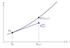
Figure 1:Forward Euler extrapolates from the current state along the initial tangent, producing a local discretization error relative to the exact trajectory.
Advantages
very simple;
fully explicit;
one vector-field evaluation per step;
easy to implement;
useful when computational resources are severely limited.
Disadvantages
only first-order accurate;
poor stability for many systems;
requires small step sizes;
accumulates significant global error;
performs poorly for stiff systems.
Local and Global Error
The local truncation error is the error made in one step assuming the starting value is exact.
For forward Euler,
The global error after many steps is
For a sufficiently smooth and stable problem,
Thus, forward Euler is globally first-order accurate.
Truncation Error and Roundoff Error
Reducing the step size decreases truncation error, but it increases the number of arithmetic operations.
Two competing effects occur:
Large step size: truncation error dominates.
Extremely small step size: roundoff and cancellation errors may dominate.
If
is smaller than machine resolution relative to , the update may numerically satisfy
even when the true solution is changing.
Backward Euler Method
Evaluate the vector field at the end of the interval:
Therefore,
This is the backward Euler method.
The method is implicit because appears on both sides.
Solving the Implicit Equation
Define the residual
At every step, solve
A fixed-point iteration is
A simple initial guess is
or a forward Euler prediction.
Newton’s method may instead be used:
The Jacobian is
Explicit and Implicit Schemes
A method is explicit if
can be computed directly from known quantities.
A method is implicit if the new state satisfies a nonlinear algebraic equation.
Explicit methods are typically cheaper per step.
Implicit methods are typically more stable and are often preferred for stiff problems.
The Generalized -Method
A unified one-step family is
Equivalently,
Special cases are:
The trapezoidal scheme is
Unlike Euler methods, it is second-order accurate.
Stability Analysis Using the Test Equation
Consider
with
The exact solution decays:
A numerical method produces
where is the stability function.
The method is stable for a given if
Forward Euler
Stability requires
For real negative ,
Therefore, the step size is restricted.
Backward Euler
Backward Euler is stable for the entire left half-plane:
It is therefore A-stable.
Trapezoidal rule
It is also A-stable, but unlike backward Euler, it does not strongly damp very fast modes.
Accuracy Versus Stability
Accuracy and stability are distinct concepts.
A method may be:
accurate but unstable for a selected step;
stable but inaccurate;
both stable and accurate; or
neither.
Backward Euler and forward Euler are both first-order accurate, but backward Euler has much stronger stability properties.
Multiple-Stage Methods
Instead of estimating the slope at only one point, multiple-stage methods estimate slopes at several locations within a step.
Runge–Kutta methods are one-step, multiple-stage methods.
They do not require values from earlier time steps beyond , but they use several vector-field evaluations during the interval
Classical Fourth-Order Runge–Kutta Method
Let
Define:
The update is
The method requires four vector-field evaluations per step.
Its global error is
Interpretation of RK4
RK4 computes:
one slope at the beginning;
two slopes near the midpoint; and
one slope at the end.
The weighted average
approximates the integrated effect of the vector field across the interval.
Computational Cost
A higher-order method typically reduces error for a given step size but requires more work per step.
The relevant cost is not simply the number of stages.
One should compare:
A fourth-order method may be cheaper overall because it permits much larger steps for the same accuracy.
The Discrete Problem Is Not the Continuous Problem
The continuous problem is
After discretization, the numerical method defines a different problem:
The step size is a parameter that does not appear in the original differential equation.
For each selected mesh, the discrete problem generally has a different solution.
Therefore, one should say:
The computation provides a numerical solution of a discrete approximation to the differential equation.
It does not provide the exact continuous solution unless a special exactness property happens to hold.
Consistency, Stability, and Convergence
Three concepts are fundamental.
Consistency
A method is consistent if the local truncation error vanishes as
Stability
A method is stable if perturbations do not grow uncontrollably under the discrete propagation.
Convergence
A method is convergent if
as the mesh is refined.
For standard linear multistep settings, consistency plus zero-stability implies convergence. For one-step methods, analogous stability and consistency results apply.
Sequential Form of Forward Euler
The forward Euler equations are:
In time marching, each equation is used after the preceding state has been computed.
Residual Form
Each equation can instead be written as a residual:
Stack the unknown states:
Stack all residuals:
This is a system of nonlinear algebraic equations.
Simultaneous Solution
Instead of computing the states sequentially, solve all state values simultaneously:
Possible root-finding methods include:
Newton’s method;
quasi-Newton methods;
trust-region methods;
nonlinear least-squares methods; and
sparse nonlinear equation solvers.
For forward Euler, sequential and simultaneous solutions are mathematically equivalent when solved exactly.
However, the simultaneous viewpoint is the conceptual bridge to direct transcription.
Backward Euler in Residual Form
Backward Euler gives
Stacking all intervals yields
The entire trajectory can be solved as one algebraic system.
This avoids performing a separate nonlinear iteration at each time step, although the global nonlinear solver still performs iterations.
Introduction to Collocation
Collocation enforces equality between:
an approximation of the derivative; and
the differential-equation vector field
at selected points.
For forward Euler:
For backward Euler:
These equations force the derivative approximation and vector field to coincide at the selected collocation point.
Defect Constraints
The residual
is often called a defect.
The discrete dynamics are enforced by
In direct optimal control, state values are optimization variables and defects become equality constraints in a nonlinear program.
Time Marching Versus Collocation
Time marching
computes states sequentially;
naturally solves initial-value problems;
propagates errors forward;
may be sensitive to unstable dynamics.
Collocation
treats many or all state values as unknowns;
enforces dynamics simultaneously;
naturally supports boundary-value problems;
integrates well with nonlinear programming;
produces sparse algebraic structures.
Connection to Direct Optimal Control
In a direct transcription method, one may optimize over:
The differential equations become algebraic defect constraints:
The objective is discretized:
Path constraints are enforced at nodes or collocation points:
Thus, the continuous optimal-control problem becomes a sparse nonlinear programming problem.
Common Errors
Calling forward Euler accurate merely because the step is small.
Ignoring roundoff when reducing the step size.
Confusing local and global truncation error.
Assuming implicit methods are automatically higher order.
Assuming stability and accuracy are the same.
Comparing methods only by the number of function evaluations.
Saying a numerical result is the exact solution of the differential equation.
Forgetting that the step size changes the discrete problem.
Treating collocation as unrelated to finite differences.
Ignoring defect convergence under mesh refinement.
Verification Guidelines
A numerical ODE solution should be checked by:
reducing the step size;
comparing multiple integration methods;
monitoring local error estimates;
checking invariants or conserved quantities;
comparing with analytic solutions when available;
evaluating residuals;
inspecting stability restrictions;
testing variable-step methods;
checking sensitivity to tolerances; and
documenting convergence rates.
Summary
The main conclusions are:
Numerical integration approximates a continuous ODE on a discrete mesh.
Forward Euler is explicit, simple, and first-order accurate.
Backward Euler is implicit, first-order accurate, and much more stable.
The -method unifies forward Euler, backward Euler, and trapezoidal integration.
RK4 uses four stages and provides fourth-order global accuracy.
Truncation, roundoff, stability, and cost must all be balanced.
A discretized equation is a different mathematical problem from the original ODE.
Time-marching equations can be rewritten as simultaneous algebraic residuals.
Enforcing derivative approximations and vector fields at common points leads to collocation.
Collocation is a central foundation of direct numerical optimal-control methods.
Connection. A time-marching formula can be imposed simultaneously rather than sequentially; Euler collocation makes this algebraic viewpoint explicit.