Chapter 6: Open-Loop Optimal Control in CCD

Discovering physical performance limits¶

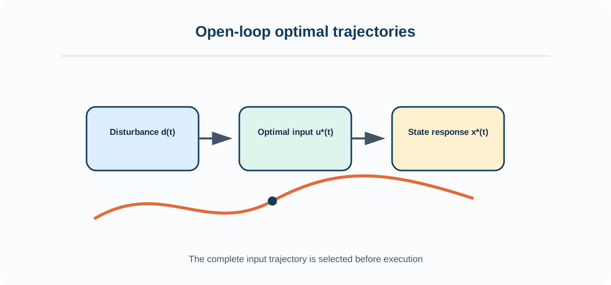
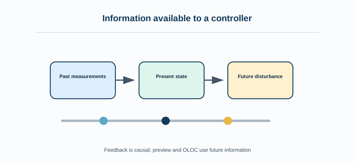
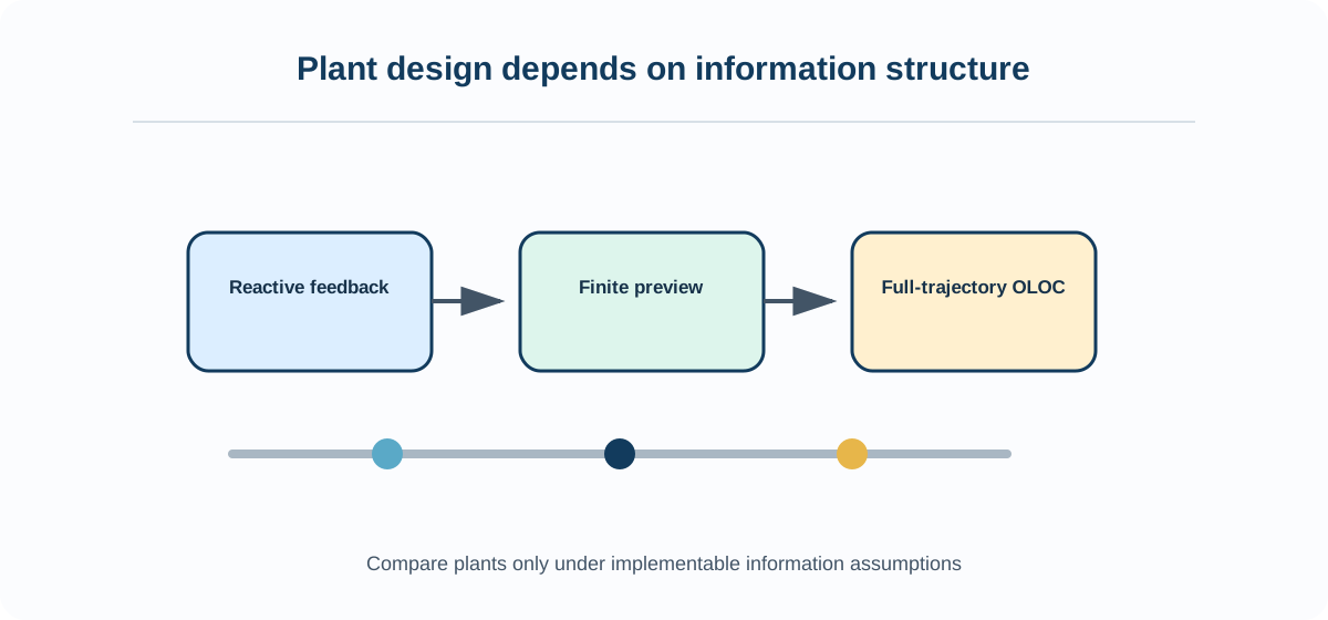
Open-loop CCD reveals performance limits, actuator requirements, active constraints, and unexpected operating phases with few controller-structure assumptions. Its optimized input generally uses information unavailable to a causal controller.

Learning objectives¶

After completing this chapter, you should be able to:

1. explain and apply plant variables;

2. explain and apply known disturbance;

3. explain and apply optimal control;

4. explain and apply state response;

5. formulate and verify the chapter methods on an active suspension with complete road preview and a wave-energy converter with known future waves.

Mathematical lens¶

The recurring quantities are $p$, $u(t)$, $x(t)$, and known $d(t)$:

Running example¶

The recurring example is an active suspension with complete road preview and a wave-energy converter with known future waves. Retaining one system prevents apparent improvements from being caused by changed physics, information, loads, or metrics.

Recommended workflow¶

1. state information assumption.

2. optimize trajectory.

3. identify phases.

4. perturb model and input.

5. translate insight to feedback.

Chapter map¶

1. What Open-Loop Optimal Control Means

2. Open-Loop Single-Control Formulations

3. Open-Loop Multiple-Control Formulations

4. Control-Vector Parameterization

5. State and Control Path Constraints

6. Free Initial and Final Times

7. Interpreting Optimal Trajectories

8. OLOC as a Performance Upper Bound

9. Sensitivity to Disturbances and Model Error

10. Why an OLOC-Optimal Plant May Not Be Closed-Loop Optimal