Chapter 10: Numerical Optimal Control for CCD

Converting time-dependent design problems into solvable optimization problems¶

Numerical optimal control replaces functions of time with finite decision vectors while preserving dynamics and constraints to a chosen accuracy. Representation, defects, sparsity, scaling, and mesh convergence drive reliability.

Learning objectives¶

After completing this chapter, you should be able to:

1. explain and apply continuous problem;

2. explain and apply time mesh;

3. explain and apply state and control samples;

4. explain and apply defect equations;

5. formulate and verify the chapter methods on minimum-time mass–spring motion, a suspension road event, and a two-phase energy converter.

Mathematical lens¶

The recurring quantities are discrete $X$, $U$, plant $p$, and possibly final time:

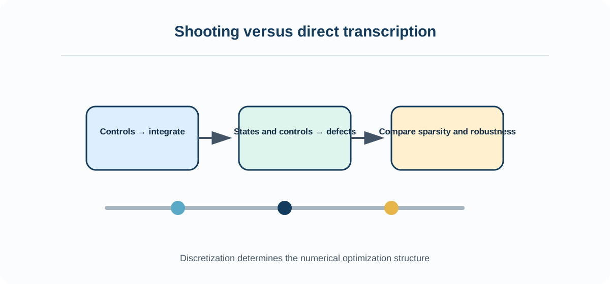
Running example¶

The recurring example is minimum-time mass–spring motion, a suspension road event, and a two-phase energy converter. Retaining one system prevents apparent improvements from being caused by changed physics, information, loads, or metrics.

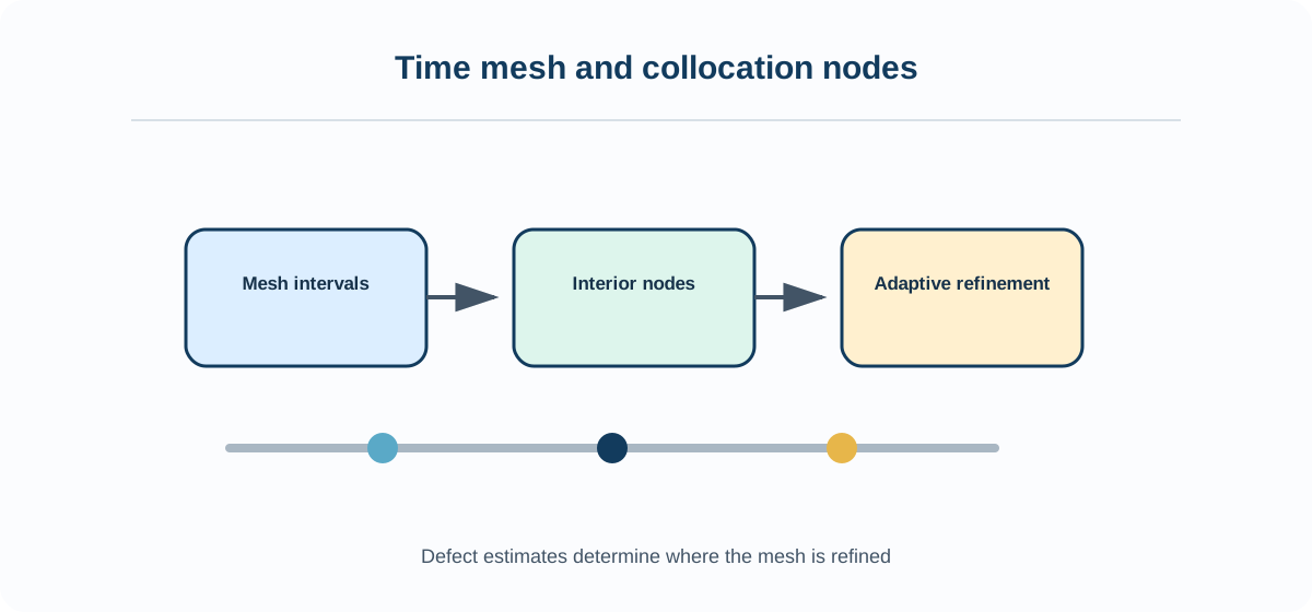
Recommended workflow¶

1. choose transcription.

2. initialize mesh.

3. solve NLP.

4. estimate error.

5. refine and verify.

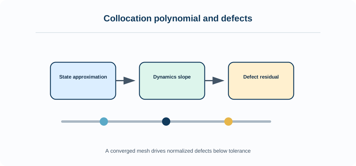
Chapter map¶

1. Indirect and Direct Methods

2. Direct Single Shooting

3. Multiple Shooting

4. Control-Vector Parameterization

5. Direct Transcription

6. Trapezoidal and Hermite–Simpson Methods

7. Gaussian Collocation

8. LG, LGR, and LGL Pseudospectral Methods

9. Mesh Refinement

10. Multiphase Problems

11. Choosing a Transcription Method