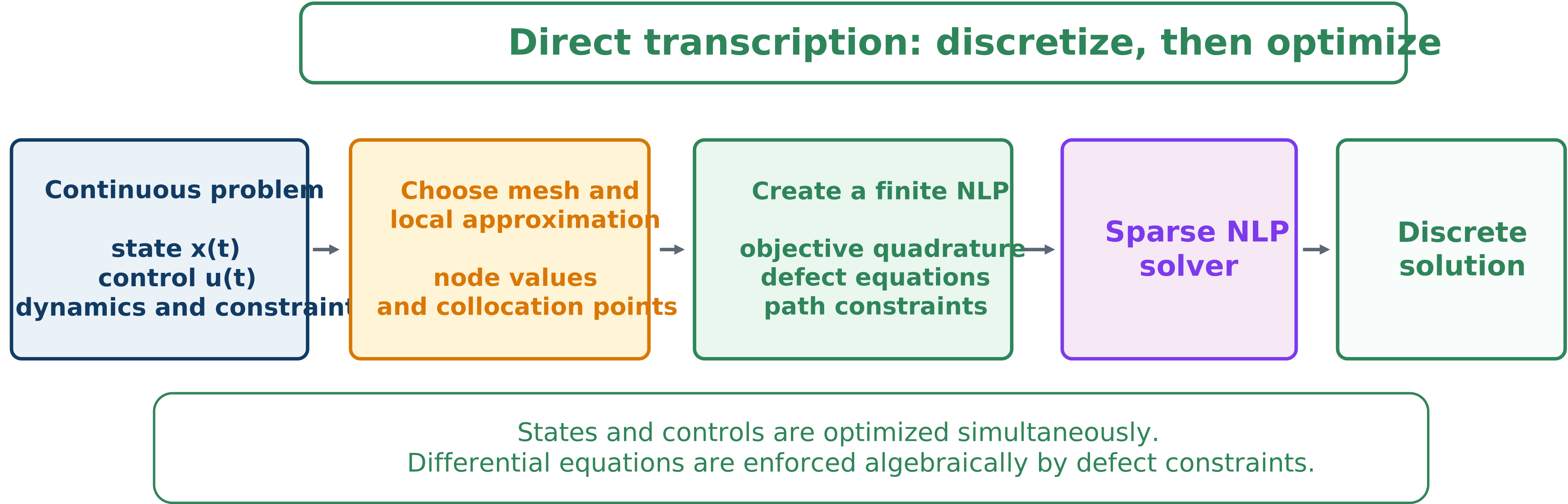
Direct Transcription
Direct transcription treats state and control samples as optimization variables and replaces differential equations with algebraic defects.
Discretize first, then optimize all trajectory and design variables together.
A time-ordered decision vector may be
z = [ x p , x c , x 0 , u 0 , … , x N , u N ] T . \mathbf{z}=[\mathbf{x}_p,\mathbf{x}_c,\mathbf{x}_0,\mathbf{u}_0,\ldots,\mathbf{x}_N,\mathbf{u}_N]^T. z = [ x p , x c , x 0 , u 0 , … , x N , u N ] T . A generic transcription is
minimize z Φ ^ ( z ) + ∑ k = 0 N w k L ( x k , u k , x p , x c , t k ) subject to ζ k ( x k , u k , x k + 1 , u k + 1 , x p , x c ) = 0 , c ( x k , u k , x p , x c , t k ) ≤ 0 , b ( x 0 , x N , x p , x c ) = 0 , z L ≤ z ≤ z U . \begin{aligned}
\underset{\mathbf{z}}{\text{minimize}}\quad
&\widehat{\Phi}(\mathbf{z})+\sum_{k=0}^Nw_kL(\mathbf{x}_k,\mathbf{u}_k,\mathbf{x}_p,\mathbf{x}_c,t_k)\\
\text{subject to}\quad
&\boldsymbol{\zeta}_k(\mathbf{x}_k,\mathbf{u}_k,\mathbf{x}_{k+1},\mathbf{u}_{k+1},\mathbf{x}_p,\mathbf{x}_c)=\mathbf{0},\\
&\mathbf{c}(\mathbf{x}_k,\mathbf{u}_k,\mathbf{x}_p,\mathbf{x}_c,t_k)\leq\mathbf{0},\\
&\mathbf{b}(\mathbf{x}_0,\mathbf{x}_N,\mathbf{x}_p,\mathbf{x}_c)=\mathbf{0},\\
&\mathbf{z}^L\leq\mathbf{z}\leq\mathbf{z}^U.
\end{aligned} z minimize subject to Φ ( z ) + k = 0 ∑ N w k L ( x k , u k , x p , x c , t k ) ζ k ( x k , u k , x k + 1 , u k + 1 , x p , x c ) = 0 , c ( x k , u k , x p , x c , t k ) ≤ 0 , b ( x 0 , x N , x p , x c ) = 0 , z L ≤ z ≤ z U . Direct transcription is valuable for CCD because it handles nonlinear plant-dependent dynamics, unstable systems, strong coupling, state/control path limits, and terminal constraints while exposing local sparsity.
Activity 7.3: Plant and Actuator Co-Design of a Dynamic System 
Consider
x ˙ 1 = x 2 , m x ˙ 2 = − k x 1 − c x 2 + u , \dot{x}_1=x_2,
\qquad
m\dot{x}_2=-kx_1-cx_2+u, x ˙ 1 = x 2 , m x ˙ 2 = − k x 1 − c x 2 + u , where m = 1 m=1 m = 1 c = 0.5 c=0.5 c = 0.5 k k k F max F_{\max} F m a x
0.5 ≤ k ≤ 8 , 0.2 ≤ F max ≤ 5. 0.5\leq k\leq 8,
\qquad
0.2\leq F_{\max}\leq 5. 0.5 ≤ k ≤ 8 , 0.2 ≤ F m a x ≤ 5. The control satisfies
∣ u ( t ) ∣ ≤ F max . |u(t)|\leq F_{\max}. ∣ u ( t ) ∣ ≤ F m a x . Use
x ( 0 ) = [ 1 0 ] , x ( t f ) = [ 0 0 ] , t f = 4. \mathbf{x}(0)=
\begin{bmatrix}
1\\
0
\end{bmatrix},
\qquad
\mathbf{x}(t_f)=
\begin{bmatrix}
0\\
0
\end{bmatrix},
\qquad
t_f=4. x ( 0 ) = [ 1 0 ] , x ( t f ) = [ 0 0 ] , t f = 4. Minimize
J = ∫ 0 t f ( x 1 2 + 0.1 x 2 2 + 0.01 u 2 ) d t + 0.03 F max 2 + 0.002 k 2 . J=
\int_0^{t_f}
\left(x_1^2+0.1x_2^2+0.01u^2\right)\,dt
+0.03F_{\max}^2
+0.002k^2. J = ∫ 0 t f ( x 1 2 + 0.1 x 2 2 + 0.01 u 2 ) d t + 0.03 F m a x 2 + 0.002 k 2 . Nondimensionalize the states, control, time, and design variables.
Formulate the simultaneous direct-collocation problem.
Solve the problem using GPOPS-II or Dymos.
Determine whether the actuator constraint is active.
Repeat the solution after multiplying the F max 2 F_{\max}^2 F m a x 2
Explain how the actuator-cost weight changes both k ∗ k^* k ∗ F max ∗ F_{\max}^* F m a x ∗