Derivative Computation - Control Co-Design

Large CCD problems typically require gradient-based optimization: objective gradients, constraint Jacobians, and sometimes Lagrangian Hessians.

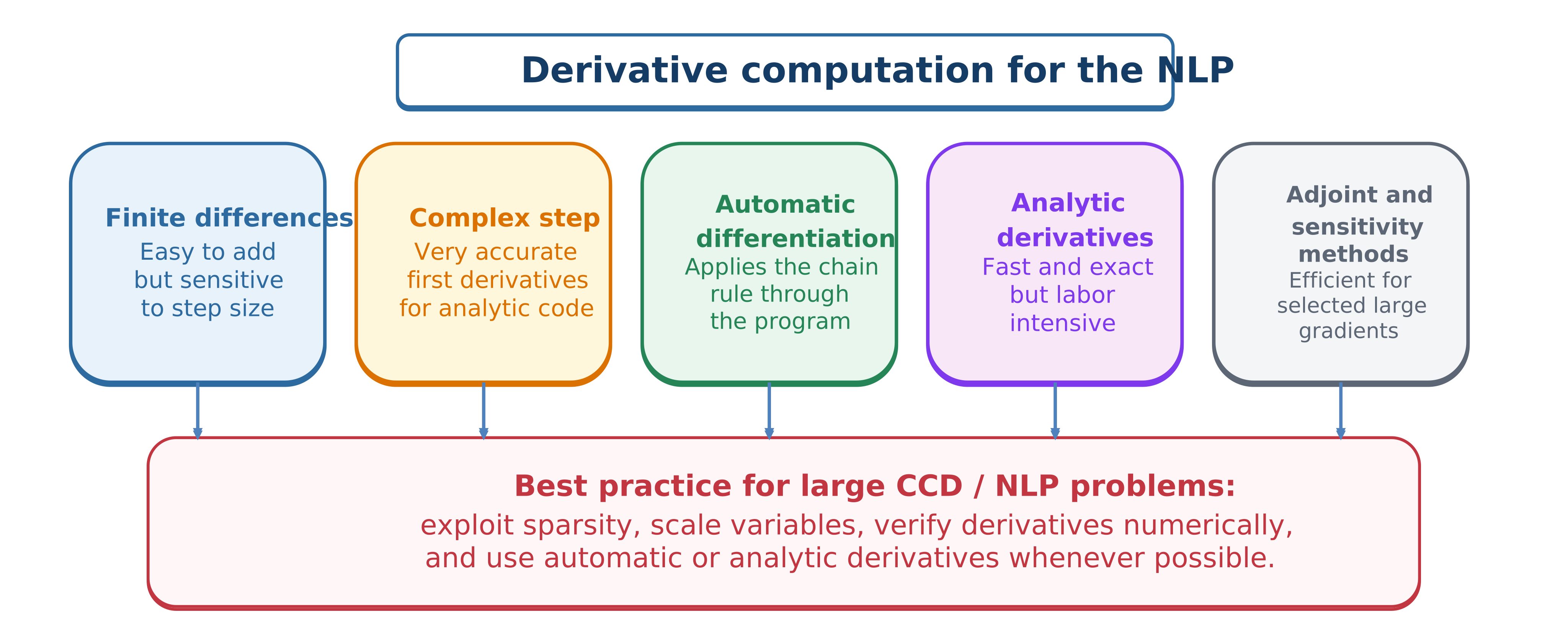
Major derivative-computation options for nonlinear programming.

Finite differences¶

\frac{\partial F}{\partial z_i}\approx\frac{F(\mathbf{z}+h\mathbf{e}_i)-F(\mathbf{z})}{h}

(1)

is easy to implement but balances truncation against cancellation and may require one evaluation per column. Sparse coloring perturbs structurally independent columns together.

Before coloring can be applied, the solver needs to know which functions depend on which variables. One practical dependency-detection technique evaluates each constraint or objective function once with a single input component set to NaN; IEEE floating-point arithmetic propagates NaN through every expression that actually depends on that component, so a single perturbed evaluation reveals an entire row of the first-derivative sparsity pattern. Repeating this for each input component (or exploiting problem structure to batch several at once) yields the full Jacobian sparsity pattern with a small number of extra function evaluations; squaring the resulting 0/1 pattern gives a conservative estimate of the Hessian sparsity. This dependency map is what lets sparse finite-differencing compute only the structurally nonzero derivative entries, and it is what makes a single transcription implementation usable with both quasi-Newton NLP solvers, which need only the gradient and constraint Jacobian, and full-Newton solvers, which additionally need the sparse Lagrangian Hessian.

Complex-step differentiation¶

For analytic code,

\frac{\partial F}{\partial z_i}\approx \frac{\operatorname{Im}F(\mathbf{z}+ih\mathbf{e}_i)}{h}.

(2)

It avoids subtractive cancellation and is excellent for verification, provided complex numbers propagate correctly and nonanalytic operations are avoided.

Analytic derivatives¶

For a trapezoidal defect,

\boldsymbol{\zeta}_k=\mathbf{x}_{k+1}-\mathbf{x}_k-\frac{h_k}{2}(\mathbf{f}_k+\mathbf{f}_{k+1}),

(3)

representative blocks are

\frac{\partial\boldsymbol{\zeta}_k}{\partial\mathbf{x}_k}=-I-\frac{h_k}{2}\mathbf{f}_{x,k}, \quad \frac{\partial\boldsymbol{\zeta}_k}{\partial\mathbf{x}_{k+1}}=I-\frac{h_k}{2}\mathbf{f}_{x,k+1},

(4)

with analogous control blocks. These formulas expose local sparsity directly.

Automatic differentiation and sensitivities¶

Automatic differentiation applies the chain rule to code and can provide machine-precision sparse Jacobians and Hessians. Forward mode suits few independent variables; reverse mode suits scalar outputs with many inputs.

Shooting derivatives often use direct or adjoint sensitivities. Direct sensitivities propagate one system per parameter; adjoints can be efficient for many parameters and few scalar outputs.

Verification¶

Compare implemented derivatives against complex step or careful finite differences at random points. A normalized discrepancy is

E_D=\frac{\|\mathbf{d}_{\mathrm{implemented}}-\mathbf{d}_{\mathrm{reference}}\|_2} {\max(1,\|\mathbf{d}_{\mathrm{reference}}\|_2)}.

(5)

Derivative errors can cause slow convergence, false convergence, or convergence to the wrong point.

Activity 7.4: Analytical Hermite--Simpson Jacobian¶

Activity 7.4: Analytical Hermite--Simpson Jacobian

Consider the nonlinear, parameter-dependent system

\dot{x}_1=x_2, \qquad \dot{x}_2=-p\sin x_1+u,

(6)

where $p$ is a plant-design variable. For interval $i$ , define

\mathbf{f}_i=\mathbf{f}(\mathbf{x}_i,u_i,p), \qquad \mathbf{f}_{i+1}=\mathbf{f}(\mathbf{x}_{i+1},u_{i+1},p),

(7)

and

\mathbf{x}_{i+1/2} =\frac{\mathbf{x}_i+\mathbf{x}_{i+1}}{2} +\frac{h_i}{8}\left(\mathbf{f}_i-\mathbf{f}_{i+1}\right).

(8)

The Hermite--Simpson defect is

\mathbf{d}_i =\mathbf{x}_{i+1}-\mathbf{x}_i -\frac{h_i}{6} \left(\mathbf{f}_i+4\mathbf{f}_{i+1/2}+\mathbf{f}_{i+1}\right).

(9)

Derive
$\frac{\partial\mathbf{d}_i}{\partial\mathbf{x}_i}, \qquad \frac{\partial\mathbf{d}_i}{\partial\mathbf{x}_{i+1}}, \qquad \frac{\partial\mathbf{d}_i}{\partial u_i}, \qquad \frac{\partial\mathbf{d}_i}{\partial u_{i+1}}, \qquad \frac{\partial\mathbf{d}_i}{\partial p}.$
(10)
Assemble the Jacobian sparsity pattern for $N$ intervals.
Determine the exact number of nonzero entries.
Explain why the column associated with $p$ is globally dense while the state and control blocks remain locally sparse.
Verify the analytical Jacobian using complex-step differentiation.

Activity 7.5: Derivative Verification for a Shooting Formulation¶

Activity 7.5: Derivative Verification for a Shooting Formulation

Consider

\dot{x}=-x^3+u, \qquad x(0)=1, \qquad 0\leq t\leq 2.

(11)

Parameterize $u(t)$ using $N=20$ piecewise-constant values:

\mathbf{U}= \begin{bmatrix} u_0 & u_1 & \cdots & u_{19} \end{bmatrix}^{T}.

(12)

Minimize

J(\mathbf{U})=x(2)^2+0.05\int_0^2u(t)^2\,dt.

(13)

Derive the forward-sensitivity equations
$\frac{d}{dt}\left(\frac{\partial x}{\partial u_j}\right) =-3x^2\frac{\partial x}{\partial u_j} +\frac{\partial u}{\partial u_j}.$
(14)
Derive the gradient $\nabla_{\mathbf{U}}J$ .
Compute the gradient using:
1. forward finite differences;
2. central finite differences;
3. complex-step differentiation; and
4. sensitivity equations or automatic differentiation.
Perform a directional-derivative test using a random normalized vector $\mathbf{p}$ .
Plot derivative error for step sizes from 10^-2 to 10^-14.
Explain the truncation-error and cancellation-error regions in the resulting plot.