Formulation and Design Variables

Why formulation matters¶

A CCD study begins as an engineering question:

What tower geometry and pitch-control tuning should reduce wind-turbine loads while maintaining power quality?

What suspension parameters and feedback gains should balance ride comfort, road holding, and actuator effort?

To turn such questions into optimization problems, we must identify:

the decision variables;
the quantity to minimize or maximize;
the physical laws the design must obey;
the engineering limits that cannot be violated; and
the time interval over which the problem applies.

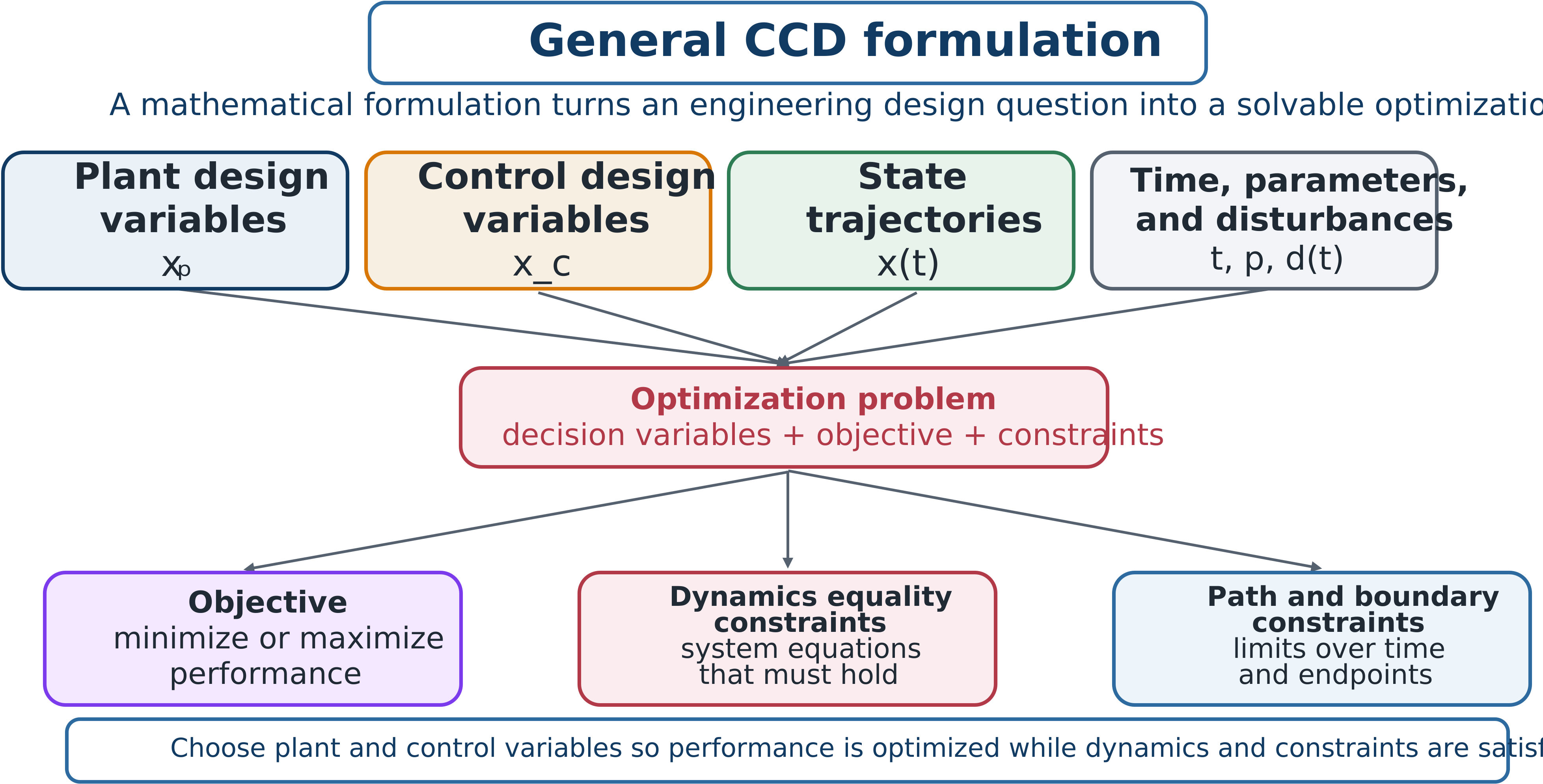
Plant and control decisions, trajectories, objective terms, dynamics, constraints, bounds, and disturbances assembled into a CCD formulation.

The main ingredients of a mathematical CCD formulation.

A formulation determines what the optimizer is allowed to do. Poorly defined variables, a misleading objective, or missing physics can produce a numerically polished but physically meaningless result.

Plant design variables¶

Plant variables describe physical-system, structural, mechanism, or hardware decisions. Denote them by

\mathbf{x}_p\in\mathbb{R}^{n_p}.

(1)

Examples include suspension stiffness and damping, structural dimensions, inertia and mass distribution, actuator or sensor placement, buoy or rotor geometry, and power-take-off parameters. These decisions often enter the dynamic model directly through mass, stiffness, damping, actuation, or output equations.

Typical examples are:

Vehicle suspension: $k_s$ , $c_s$ , and tire stiffness $k_t$ .
Robot arm: link lengths, gear ratios, motor sizes, and joint stiffness.
Wind turbine: blade properties, tower diameter, and drivetrain inertia.
Marine energy device: buoy radius, draft, PTO characteristics, and mooring stiffness.

Plant variables usually have defensible bounds,

\mathbf{x}_p^L\leq\mathbf{x}_p\leq\mathbf{x}_p^U,

(2)

reflecting manufacturability, safety, packaging, cost, and physical realism.

Control design variables¶

Control variables define how the controller behaves. Denote them by

\mathbf{x}_c\in\mathbb{R}^{n_c}.

(3)

Examples of physical plant variables and controller variables shown as two coupled decision groups.

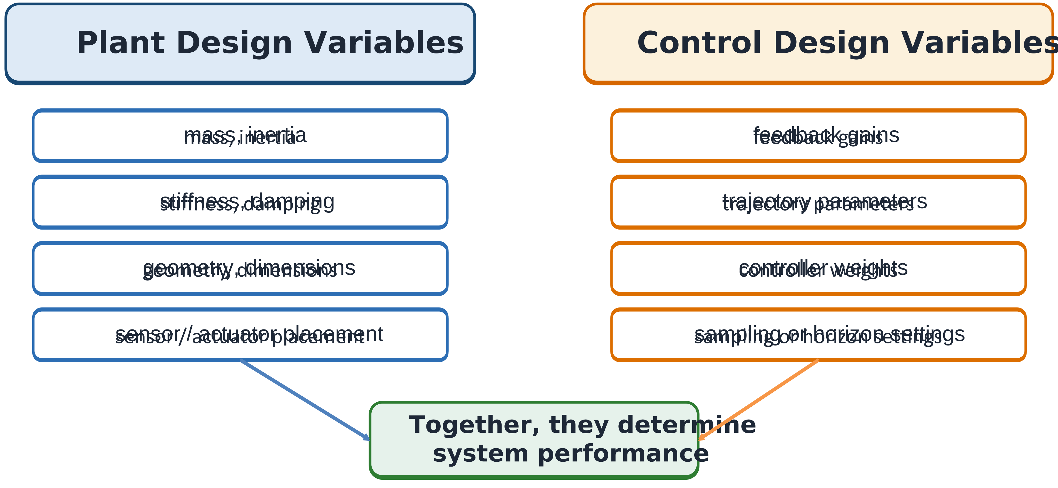
Plant and control variables are distinct, but both affect system performance and must be chosen together.

Control variables may include PID or state-feedback gains, weighting matrices, trajectory parameters, feedforward coefficients, switching thresholds, sampling times, prediction horizons, or coefficients in a control-law parameterization.

Parameterized control and free trajectories¶

There are two common control representations:

Parameterized control design: a law depends on finite parameters $\mathbf{x}_c$ , for example
$u(t)=-K(\mathbf{x}_c)x(t).$
(4)
Direct trajectory optimization: the function $u(t)$ itself is a time-varying decision.

Either can be used in CCD. The appropriate choice depends on the problem structure, intended controller implementation, and numerical method.

Partitioning the control-variable set¶

It is often useful to be explicit about which part of $\mathbf{x}_c$ is time-independent and which is a genuine trajectory. Writing

\mathbf{x}_c=\begin{bmatrix}\mathbf{p}\\\mathbf{u}\end{bmatrix},

(5)

separates control parameters $\mathbf{p}$ —time-independent quantities such as feedback gains, weighting-matrix entries, or a prediction horizon—from open-loop control (OLC) variables $\mathbf{u}(\cdot)$ , the time-varying trajectory itself. A formulation may include only $\mathbf{p}$ (a fully parameterized feedback law), only $\mathbf{u}(\cdot)$ (direct trajectory optimization with no parametric structure), or both at once, for example a parameterized feedback law whose reference trajectory is itself optimized. The general continuous-time CCD formulation developed later in this chapter accommodates all three cases without change; only the content of $\mathbf{x}_c$ differs.