Gradient-Based Optimization - Control Co-Design

The gradient¶

For a scalar objective $f(\mathbf{x})$ ,

\nabla f(\mathbf{x})= \begin{bmatrix} \partial f/\partial x_1&\partial f/\partial x_2&\cdots&\partial f/\partial x_n \end{bmatrix}^T.

(1)

The gradient points in the direction of steepest local increase in Euclidean coordinates, so $-\nabla f$ points toward steepest local decrease.

Gradient descent¶

The basic update is

\mathbf{x}_{k+1}=\mathbf{x}_k-\alpha_k\nabla f(\mathbf{x}_k),

(2)

where $\alpha_k>0$ is the step length.

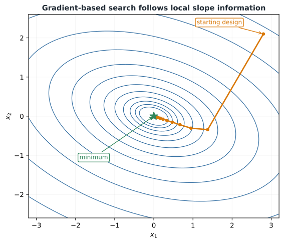
A sequence of gradient-based steps moving across objective contours toward a nearby minimum.

Each update uses local slope information. Small steps are slow, while overly large steps may overshoot or diverge.

Line search and trust regions¶

A line-search method chooses a direction $\mathbf{p}_k$ and seeks an acceptable solution to

\underset{\alpha>0}{\text{minimize}}\quad f(\mathbf{x}_k+\alpha\mathbf{p}_k).

(3)

The direction may come from steepest descent, Newton, or quasi-Newton information. A practical line search seeks sufficient reduction rather than an exact one-dimensional optimum. Trust-region methods instead restrict the step to a region where a local model is considered reliable.

Newton and quasi-Newton methods¶

A second-order Taylor approximation is

f(\mathbf{x}_k+\mathbf{p})\approx f(\mathbf{x}_k)+\nabla f(\mathbf{x}_k)^T\mathbf{p}+\frac12\mathbf{p}^TH(\mathbf{x}_k)\mathbf{p}.

(4)

Minimizing this quadratic model gives the Newton step

H(\mathbf{x}_k)\mathbf{p}_k=-\nabla f(\mathbf{x}_k).

(5)

Newton’s method can converge rapidly near a well-behaved optimum, but exact Hessians may be expensive and the step may fail if the Hessian is indefinite or ill-conditioned. Quasi-Newton methods such as BFGS estimate Hessian information from changes in gradients.

Computing derivatives¶

Gradient-based algorithms are only as reliable as the derivatives they receive. Four practical families of methods exist, and they differ in cost, accuracy, and required access to the model.

Finite differences. The forward-difference formula follows from a truncated Taylor series,

\frac{\partial f}{\partial x_j}=\frac{f(\mathbf{x}+h\hat{e}_j)-f(\mathbf{x})}{h}+O(h),

(6)

which is first-order accurate; a central difference reaches $O(h^2)$ at roughly twice the cost. Finite differences face a step-size dilemma: shrinking $h$ reduces truncation error, but below a certain size subtractive cancellation in finite-precision arithmetic dominates and the estimate degrades—for double precision, the best forward-difference step is typically near 10^-8. Because each design direction requires a separate perturbed model evaluation, the cost of a full Jacobian scales linearly with the number of design variables. Finite differences require no access to source code, so they remain the default when a model is a black box, but they are neither the most accurate nor the most efficient option when the model can be modified.

Complex-step differentiation. Perturbing a design variable along the imaginary axis instead of the real axis,

\frac{\partial f}{\partial x_j}=\frac{\operatorname{Im}\big(f(\mathbf{x}+ih\hat{e}_j)\big)}{h}+O(h^2),

(7)

avoids subtraction entirely, so there is no cancellation error. The step size can then be shrunk toward machine precision (values near 10^-200 are typical) without any loss of accuracy, so the resulting derivative matches the precision of the function itself. The cost still scales linearly with the number of design variables, comparable to a central difference, but the method requires source-code access and correct handling of complex arithmetic (including redefined absolute-value and comparison logic).

Algorithmic (automatic) differentiation. AD applies the chain rule mechanically to every elementary operation in the source code, without ever forming a symbolic expression. In forward mode, one input is seeded and its derivative is propagated through every subsequent line of code, so the cost scales with the number of inputs and is independent of the number of outputs. In reverse mode, one output is seeded and its derivative is propagated backward to every variable it depends on, so the cost scales with the number of outputs and is independent of the number of inputs—but it requires storing intermediate values from a forward pass before the backward sweep can run. Reverse-mode AD is therefore especially attractive when a problem has many design variables and few objectives or constraints, which is common in large CCD problems.

Direct and adjoint sensitivity methods. When a model is expressed as governing residual equations, implicit differentiation of the residuals with respect to the states yields a linear system whose solution gives the total derivatives. Solving that system once per design variable is the direct method; solving it once per output is the adjoint method—mirroring the forward/reverse trade-off of AD, but applied at the level of the governing equations rather than lines of code.

Example 3.2: quadratic minimization¶

Consider

f(x_1,x_2)=2x_1^2+x_1x_2+x_2^2-6x_1-5x_2.

(8)

Its gradient is

\nabla f=\begin{bmatrix}4x_1+x_2-6\\x_1+2x_2-5\end{bmatrix}.

(9)

Setting $\nabla f=0$ gives $x_1^*=1$ and $x_2^*=2$ . The Hessian

H=\begin{bmatrix}4&1\\1&2\end{bmatrix}

(10)

is positive definite, so this stationary point is the unique global minimum of the convex quadratic.