Optimization of Dynamic Systems

Why dynamic optimization is different¶

In static optimization, the model returns quantities for one design condition. In dynamic optimization, the model generates trajectories over time. Objectives and constraints may depend on the entire trajectory rather than on one scalar state.

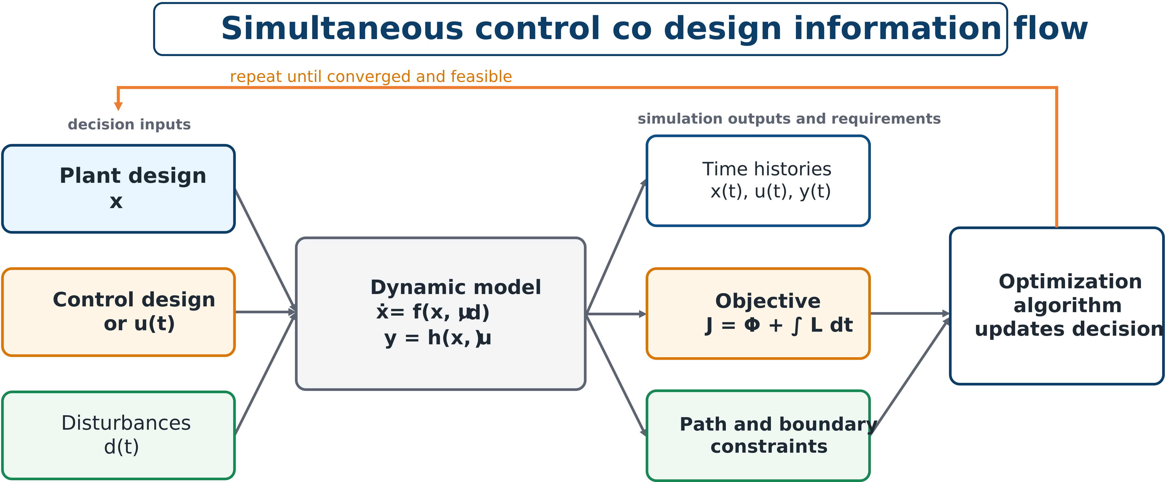
Optimization of a dynamic system: design decisions enter the model, whose time histories determine performance and feasibility.

General formulation¶

A dynamic optimization problem can be written as

The objective combines a terminal term $\Phi$, such as final error or energy, and an integral term $L$, such as accumulated tracking error, fatigue, energy, or control effort.

Path and boundary constraints¶

Path constraints must hold throughout the time interval:

Examples include actuator, displacement, temperature, contact-force, power, and stress limits. A violation may occur between sampled times, so the discretization must be fine enough to detect it.

Boundary constraints apply at the initial or final time, for example

Simulation-based optimization¶

A common workflow is to select design variables, simulate the dynamic model, compute objectives and constraints from the resulting trajectories, and return them to the optimizer. This works naturally when control is parameterized by a few variables. Optimizing an entire control trajectory requires specialized optimal-control transcription methods.

A small CCD formulation¶

For

let $c$, $k$, $K_p$, and $K_d$ be decisions and use $u=-K_pq-K_d\dot{q}$. One possible objective is

Possible constraints include $|q(t)|\leq q_{\max}$, $|u(t)|\leq u_{\max}$, and bounds on $c$, $k$, $K_p$, and $K_d$. This is already a CCD problem because plant and controller variables are optimized together.

Activity 3.6: Discrete Adjoint Sensitivities for Simulation-Based Optimization¶