Stability and Feedback - Control Co-Design

Equilibrium points¶

An equilibrium point is a state at which the system can remain indefinitely if the input is held appropriately and no perturbation moves it away. For

\dot{\mathbf{x}}=\mathbf{f}(\mathbf{x},\mathbf{u}),

(1)

a pair $(\mathbf{x}_e,\mathbf{u}_e)$ is an equilibrium if

\mathbf{f}(\mathbf{x}_e,\mathbf{u}_e)=\mathbf{0}.

(2)

For the uncontrolled mass–spring–damper system with no disturbance, the origin $(x,\dot{x})=(0,0)$ is an equilibrium.

What stability means¶

Engineers often explain stability informally:

If a small perturbation leaves the system near the equilibrium, the equilibrium is stable.
If the system returns to the equilibrium, it is asymptotically stable.
If trajectories move away, the equilibrium is unstable.

For an LTI system, these questions reduce to the eigenvalues of the matrix $A$ . For

\dot{\mathbf{x}}=A\mathbf{x},

(3)

the origin is:

asymptotically stable if every eigenvalue of $A$ has strictly negative real part;
unstable if any eigenvalue has positive real part; and
potentially marginally stable, or in need of a more careful test, when eigenvalues lie on the imaginary axis.

For the mass–spring–damper state matrix

A=\begin{bmatrix}0&1\\-k/m&-c/m\end{bmatrix},

(4)

the characteristic equation is

\lambda^2+\frac{c}{m}\lambda+\frac{k}{m}=0.

(5)

If $m>0$ , $c>0$ , and $k>0$ , the eigenvalues have negative real part and the equilibrium is asymptotically stable.

Natural frequency and damping ratio¶

For a second-order system,

\omega_n=\sqrt{\frac{k}{m}}, \qquad \zeta=\frac{c}{2\sqrt{km}}.

(6)

The natural frequency $\omega_n$ measures the speed of the undamped oscillatory dynamics, while the damping ratio $\zeta$ measures damping relative to critical damping. Greater stiffness generally raises natural frequency, greater damping raises damping ratio, and greater mass tends to lower natural frequency.

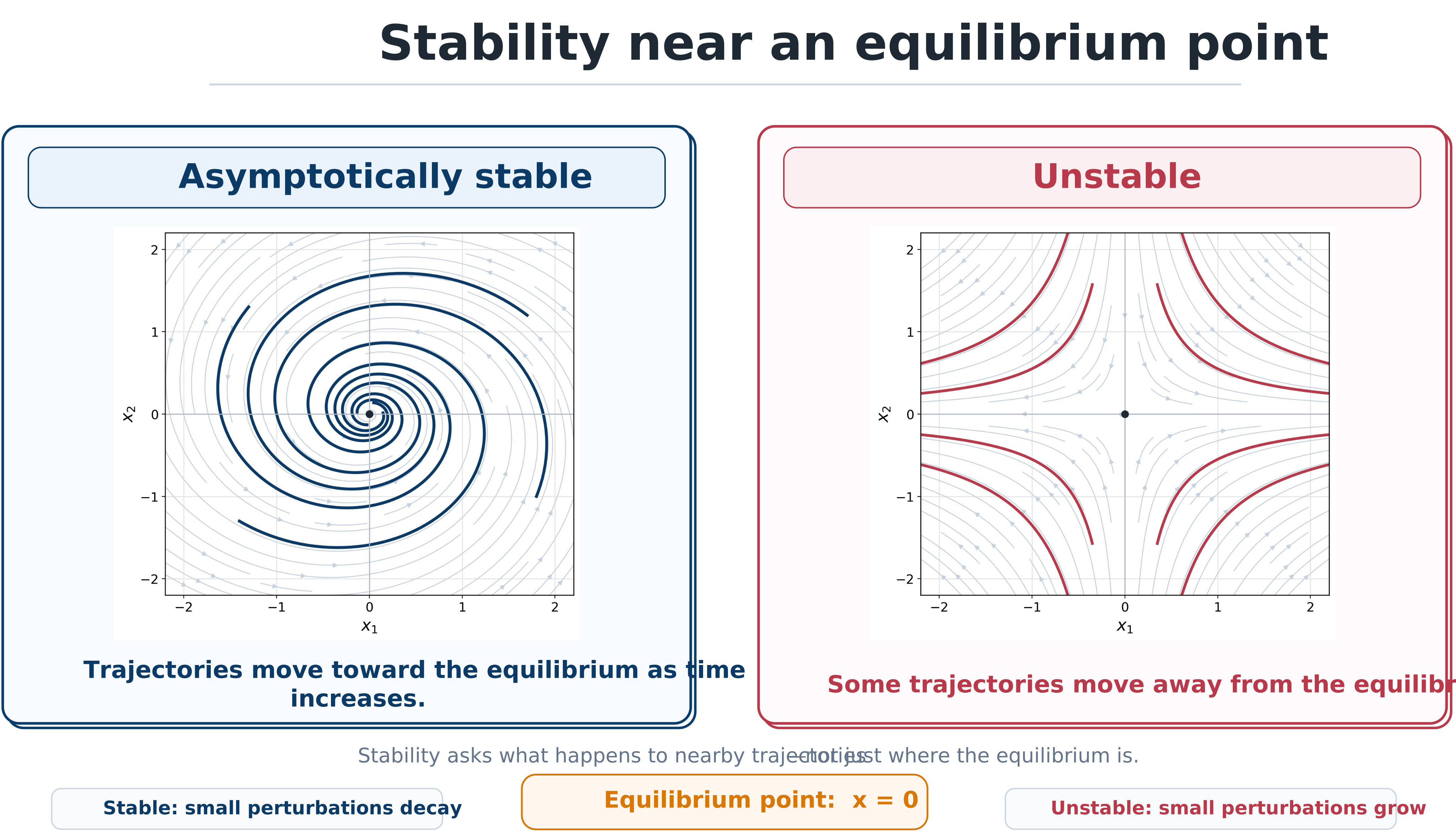
Phase-plane trajectories for asymptotically stable and unstable systems.

Stability is ultimately about trajectories. Nearby trajectories approach an asymptotically stable equilibrium, while some trajectories move away from an unstable equilibrium.

How feedback changes dynamics¶

Consider

\dot{\mathbf{x}}=A\mathbf{x}+B\mathbf{u}.

(7)

With state feedback

\mathbf{u}=-K\mathbf{x},

(8)

the closed-loop system becomes

\dot{\mathbf{x}}=(A-BK)\mathbf{x}.

(9)

Feedback reshapes the effective dynamics by changing the system matrix from $A$ to $A-BK$ .

Conceptual pole maps showing how feedback shifts closed-loop poles and changes stability and response.

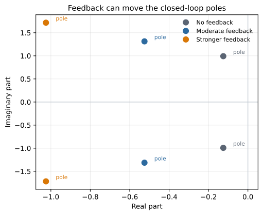
Increasing feedback can shift the closed-loop poles. Pole movement changes response speed, oscillation, and stability margin.

If the plant design changes $A$ or $B$ , the same feedback matrix $K$ no longer produces the same dynamics. Conversely, if $K$ changes, the value of a plant design may change.

A proportional–derivative example¶

For the mass–spring–damper system, choose

u(t)=-K_p x(t)-K_d\dot{x}(t).

(10)

Substituting this law into (4) gives

m\ddot{x}(t)+(c+K_d)\dot{x}(t)+(k+K_p)x(t)=d(t).

(11)

The proportional term behaves like added stiffness and the derivative term behaves like added damping. The controller can improve performance, but only through the plant to which it is attached.

Activity 2.4: Lyapunov Analysis of a Nonlinear Feedback System¶

Activity 2.4: Lyapunov Analysis of a Nonlinear Feedback System

Consider the nonlinear oscillator

m\ddot{x}+c\dot{x}+kx+\alpha x^3=u,

(12)

where

m>0, \qquad \alpha>0.

(13)

Apply the PD controller

u=-K_px-K_d\dot{x}.

(14)

Write the nonlinear closed-loop state-space model using
$x_1=x, \qquad x_2=\dot{x}.$
(15)
Determine all equilibrium points as functions of $k+K_p$ .
Consider the candidate Lyapunov function
$V(x_1,x_2) =\frac{1}{2}mx_2^2 +\frac{1}{2}(k+K_p)x_1^2 +\frac{1}{4}\alpha x_1^4.$
(16)
Derive $\dot{V}$ along closed-loop trajectories.
Prove global asymptotic stability of the origin when
$k+K_p>0, \qquad c+K_d>0.$
(17)
Explain what changes when
$k+K_p<0.$
(18)
Determine the additional equilibria and classify them locally.
Replace the ideal controller with
$u=\operatorname{sat}\left(-K_px-K_d\dot{x},F_{\max}\right).$
(19)
Derive the region in the $(x,\dot{x})$ plane in which the actuator remains unsaturated:
$|K_px+K_d\dot{x}|\leq F_{\max}.$
(20)
Find the largest Lyapunov sublevel set
$\Omega_\rho =\left\{(x,\dot{x}):V(x,\dot{x})\leq\rho\right\}$
(21)
that is guaranteed to lie inside the unsaturated region.
Verify the analytical stability conclusions numerically for at least four initial conditions inside and outside $\Omega_\rho$ .
Explain why local linear eigenvalues cannot establish the global stability properties obtained from the Lyapunov analysis.