Open-Loop and Closed-Loop Systems

Open-loop operation¶

An open-loop controller generates a command without using measurements to correct its action during operation. It may use a model or a planned trajectory, but it does not adapt to actual measured output in real time.

Open-loop control can work well when:

• the model is accurate;

• disturbances are negligible;

• repeatability is high; and

• performance requirements are modest.

Examples include timed traffic lights, simple washing-machine cycles, or a precomputed robot motion in a highly predictable setting.

Closed-loop operation¶

A closed-loop controller uses measurements to compare what is happening with what should happen and adjusts the input accordingly. Feedback can:

• reject disturbances;

• reduce sensitivity to modeling error;

• stabilize unstable or weakly damped plants; and

• improve tracking and regulation.

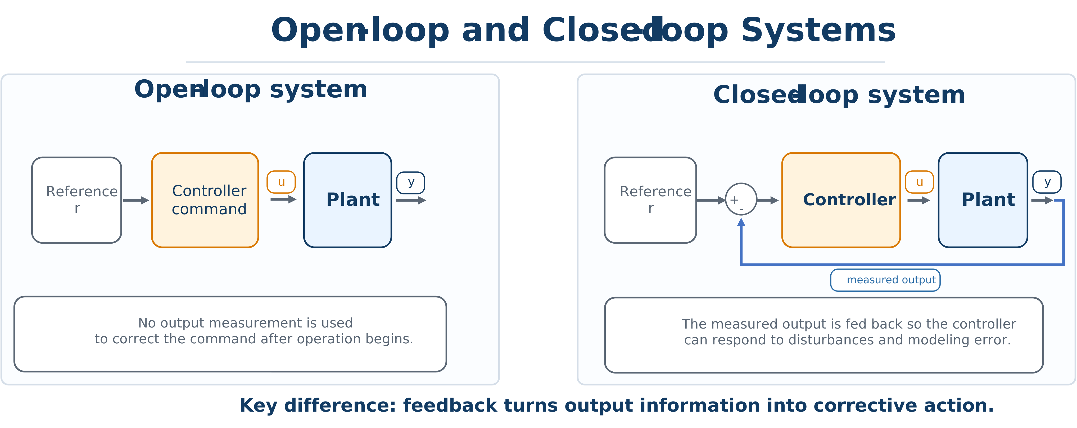
Open-loop and closed-loop structures. Closed-loop control feeds measured output back to the controller so commands can be corrected in real time.

What is actually being designed: trajectories versus gains¶

The open-loop/closed-loop distinction changes more than implementation detail — it changes what a “control design” even consists of. With no feedback mechanism, an open-loop control design is typically an entire time trajectory chosen in advance: for instance, the torque history commanded to a robotic-manipulator joint over a fixed motion, decided once and executed without regard to how the joint actually behaves along the way. With a feedback mechanism in place, a closed-loop control design instead consists of the parameters of that mechanism — gains, an observer, or another rule that maps the currently available information into an action — such as the gain matrix $K$ in the state-feedback law (8), or the gain matrices of an infinite-horizon linear-quadratic regulator using full-state feedback.

This distinction carries directly into CCD problem formulations. An open-loop CCD problem optimizes a plant together with a control trajectory $\mathbf u(\cdot)$; a closed-loop CCD problem optimizes a plant together with a feedback rule (a gain matrix, or more generally the map $\mathcal K$ from available information to a command). The two are not interchangeable: a plant tuned around a fixed, precomputed trajectory can look very different from a plant tuned to work well under a feedback law that has to react to whatever the system actually does.

Error-driven feedback¶

A standard feedback idea is to compute an error

where $r(t)$ is a reference and $y(t)$ is the measured output. The controller then uses $e(t)$ or the measured state to choose the command. In its simplest form, this may be proportional control,

More advanced architectures include proportional–integral–derivative (PID), state feedback, observer-based feedback, and model predictive control.

Why open-loop control often fails in practice¶

Suppose an open-loop command for a mass–spring–damper system is designed using nominal parameters. If the actual mass is slightly larger or the disturbance differs from the prediction, the motion may deviate from its intended path. A feedback controller corrects based on what actually happens, not only on what was predicted.